1 Payoff functions
The payoff is the cash realized by the holder of an option or other asset at the end of its life.
1.1 European options
It is often useful to characterize a European option in terms of its payoff to the purchaser of the option. The initial cost of the option is then not included in the calculation. The payoff functions for European options are the following.
- Payoff from a long position in a European call option: \(c^{+} = \mathrm{max}(S_T-K, 0)\). Or equivalently: \(c^{+}=-\mathrm{min}(K-S_T, 0)\).
- Payoff to the holder of a short position in the European call option: \(c^{-}=\mathrm{min}(K-S_T, 0)\). Or equivalently: \(c^{-}=-\mathrm{max}(S_T-K, 0)\).
- Payoff to the holder of a long position in a European put option: \(p^{+}=\mathrm{max}(K-S_T, 0)\). Or equivalently: \(p^{+}=-\mathrm{min}(S_T-K, 0)\).
- Payoff from a short position in a European put option: \(p^{-}=\mathrm{min}(S_T-K, 0)\). Or equivalently: \(p^{-}=-\mathrm{max}(K-S_T, 0)\).
Options are zero sum games because the payoffs to the holder or a long position and to the holder of a short position offset each other.
In the case of a call option:
\(c^{+}+c^{-}=\mathrm{max}(S_T-K, 0) + \mathrm{min}(K-S_T, 0)\),
\(\rightarrow c^{+}+c^{-}=\mathrm{max}(S_T-K, 0) - \mathrm{max}(S_T-K, 0)\),
\(\rightarrow c^{+}+c^{-}=0\).
In the case of a put option:
\(p^{+}+p^{-}=\mathrm{max}(K-S_T, 0) + \mathrm{min}(S_T-K, 0)\),
\(\rightarrow p^{+}+p^{-}=\mathrm{max}(K-S_T, 0) - \mathrm{max}(K-S_T, 0)\),
\(\rightarrow p^{+}+p^{-}=0\).
Graphically (assuming \(K=\$75\)):
Code
par(mfrow = c(2, 2), mai = c(0.7, 0.4, 0.4, 0.4))
par(pty = "s")
plot(ST.seq, cl, type = "l", ylim = c(0, 150), lwd = 4,
     ylab = "Payoff", xlab = "")
legend("topleft", legend = c("Long call"),
       bg = "white", bty = "n")
par(pty = "s")
plot(ST.seq, pl, type = "l", ylim = c(0, 150), lwd = 4,
     ylab = "", xlab = "")
legend("topleft", legend = c("Long put"),
       bg = "white", bty = "n")
par(pty = "s")
plot(ST.seq, cs, type = "l", ylim = c(-150, 0), lwd = 4,
     ylab = "Payoff", xlab = expression(paste(S[T])))
legend("bottomleft", legend = c("Short call"),
       bg = "white", bty = "n")
par(pty = "s")
plot(ST.seq, ps, type = "l", ylim = c(-150, 0), lwd = 4,
     ylab = "", xlab = expression(paste(S[T])))
legend("bottomleft", legend = c("Short put"),
       bg = "white", bty = "n")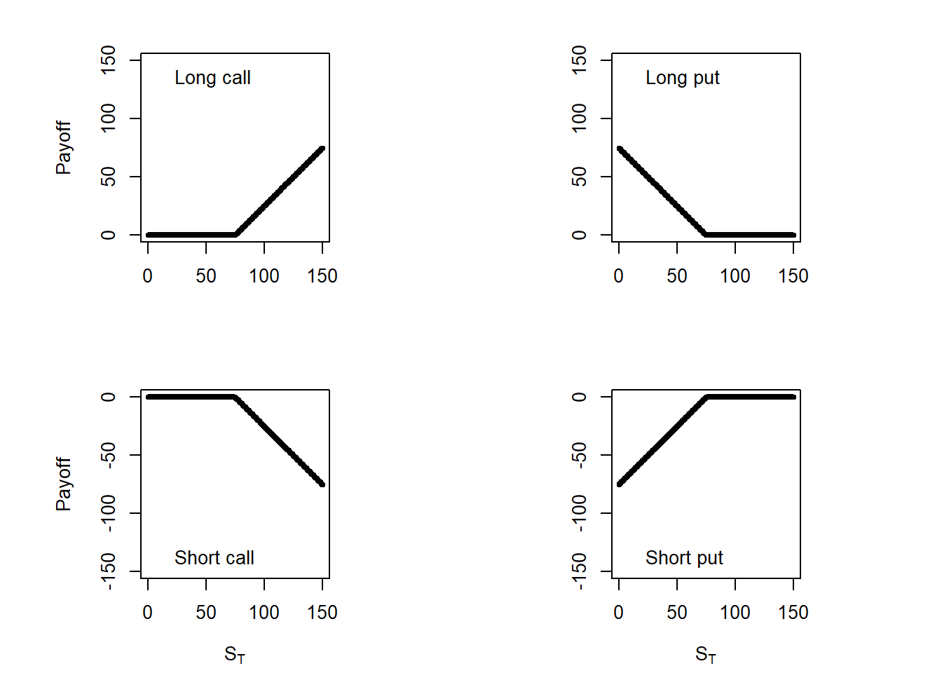
1.2 Stocks
For stocks, the diagrams below track profit from the initial stock price. The terminal cash flow from holding one share is \(S_T\); subtracting \(S_0\) turns the expression into a profit measure.
Profit from a long position in a stock: \(S_T-S_0\).
Profit from a short position in a stock: \(S_0-S_T\).
Graphically:
Code
S0 = 75
par(pty = "s")
par(mfrow = c(1, 2), oma = c(0, 0, 2, 0))
par(pty = "s")
# Long position
plot(ST.seq, ST.seq-S0, type = "l", ylab = "Profit", main = "Long stock",
     xlab = expression(paste(S[T])), lwd = 4, col = "blue",
     ylim = c(-75, 75))
abline(h = 0, lty = 2)
abline(v = 0, lty = 2)
par(pty = "s")
# Short position
plot(ST.seq, S0-ST.seq, type = "l", ylab = "", main = "Short stock",
     xlab = expression(paste(S[T])), lwd = 4, col = "red",
     ylim = c(-75, 75))
abline(h = 0, lty = 2)
abline(v = 0, lty = 2)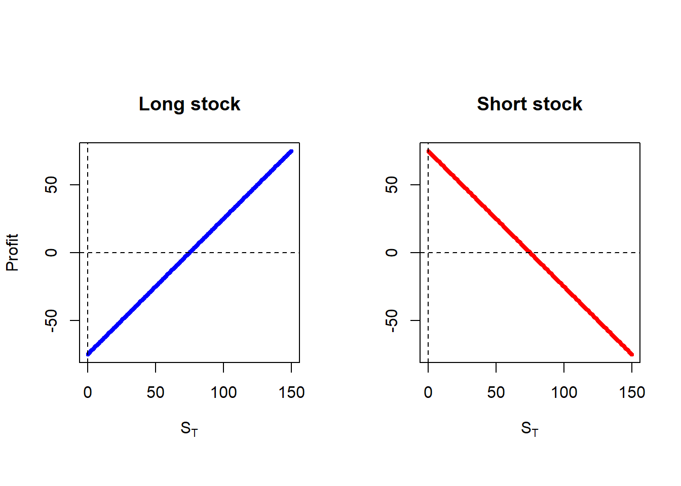
1.3 Bonds
The payoff functions for zero coupon bonds are the following.
Long position in a bond: \(K\).
Short position in a bond: \(-K\).
Graphically (assuming \(K=\$75\)):
Code
K = 75
par(pty = "s")
par(mfrow = c(1, 2), oma = c(0, 0, 2, 0))
par(pty = "s")
# Long position
plot(ST.seq, rep(K, 150), type = "l", ylab = "Payoff", main = "Long bond",
     xlab = expression(paste(S[T])), lwd = 4, col = "blue",
     ylim = c(0, 150))
abline(h = 0, lty = 2)
abline(v = 0, lty = 2)
par(pty = "s")
# Short position
plot(ST.seq, rep(-K, 150), type = "l", ylab = "", main = "Short bond",
     xlab = expression(paste(S[T])), lwd = 4, col = "red",
     ylim = c(-150, 0))
abline(h = 0, lty = 2)
abline(v = 0, lty = 2)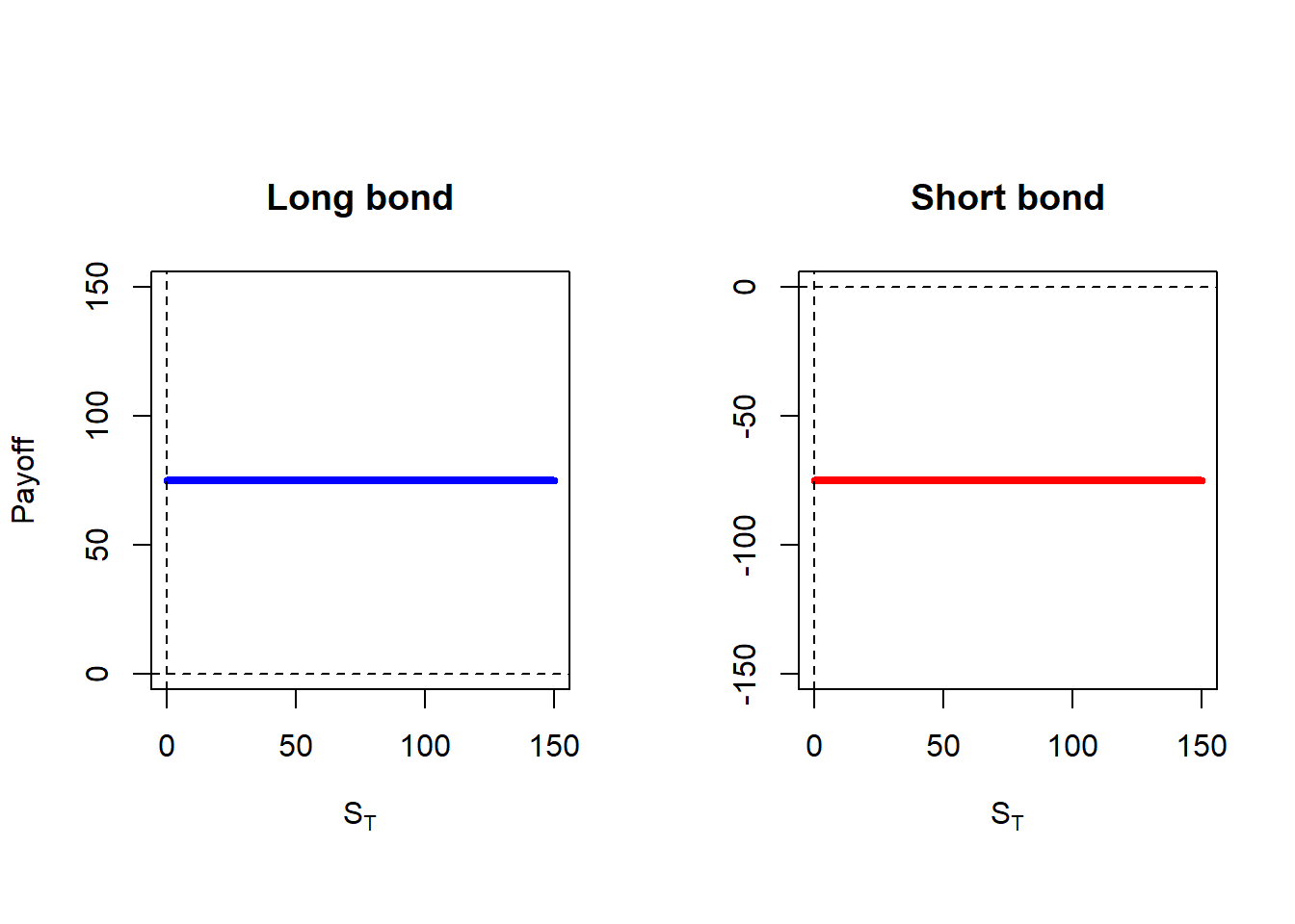
1.4 Options, stocks and bonds
We look at what can be achieved when an option is traded in conjunction with other assets. In particular, we examine the properties of portfolios consisting of (a) an option and a zero-coupon bond, (b) an option and the asset underlying the option, and (c) two or more options on the same asset. This section is based in Hull (2015) chapter 12, you can also see Brealey et al. (2020).
Code
S0 = 65
# Here I assume the stock price is currently 65.
Sl <- ST.seq - S0
# I assume the option price is 5.
cs.pr <- pmin(K - ST.seq, 0) + 5
# A short put profit is replicated by taking a short call and a long stock.
ans <- cs.pr + Sl
par(pty = "s")
plot(ST.seq, ans, type = "l", ylim = c(-75, 75), lwd = 2, col = "red",
     xlab = expression(paste(S[T])),
     ylab = "Profit")
lines(ST.seq, Sl, lty = 2, lwd = 2, col = "orange")
lines(ST.seq, cs.pr, lty = 2, lwd = 2, col = "blue")
abline(v = 0)
abline(h = 0)
abline(v = 65, lty = 2, col = "grey")
abline(v = 75, lty = 2, col = "grey")
abline(v = 80, lty = 2, col = "grey")
legend("topleft", legend = c("Short call", "Long stock", "Short put"),
       col = c("blue", "orange", "red"), lty = c(2, 2, 1),
       lwd = 2, bg = NULL)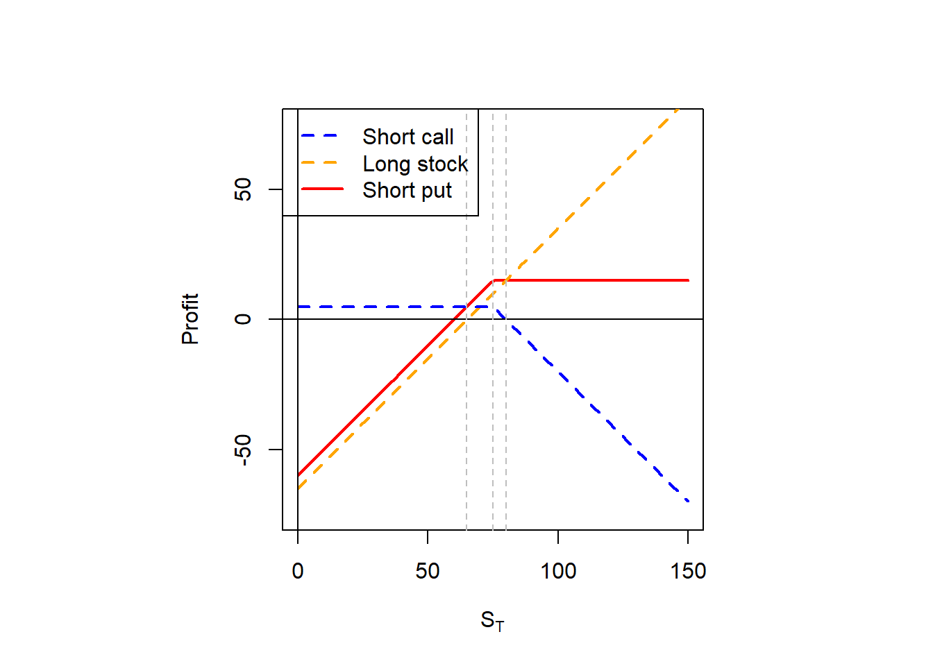
Code
S0 = 65
c_price = 5
# Here I assume the stock price is currently 65.
Sl <- ST.seq - S0
# I assume the option price is 5.
cs.pr <- pmin(K - ST.seq, 0) + c_price
# A short put profit is replicated by taking a short call and a long stock.
ans <- cs.pr + Sl
par(pty = "s")
plot(ST.seq, ans, type = "l", ylim = c(-5, 15), xlim = c(60, 80),
     lwd = 4, col = "red",
     xlab = expression(paste(S[T])),
     ylab = "Profit")
lines(ST.seq, Sl, lwd = 4, col = "orange")
lines(ST.seq, cs.pr, lwd = 4, col = "blue")
abline(v = 0)
abline(h = 0)
abline(v = 65, lty = 2, col = "grey")
abline(v = 75, lty = 2, col = "grey")
abline(v = 80, lty = 2, col = "grey")
points(S0 - c_price, 0, cex = 3, col = "red", lwd = 3)
points(K, K - S0 + c_price, cex = 3, col = "red", lwd = 3, pch = 0)
points(K + c_price, 0, cex = 3, col = "blue", lwd = 3)
points(K, c_price, cex = 3, col = "blue", lwd = 3, pch = 0)
points(S0, 0, cex = 3, col = "orange", lwd = 3)
points(K, K - S0, cex = 3, col = "orange", lwd = 3, pch = 0)
points(K, 0, cex = 3, lwd = 3)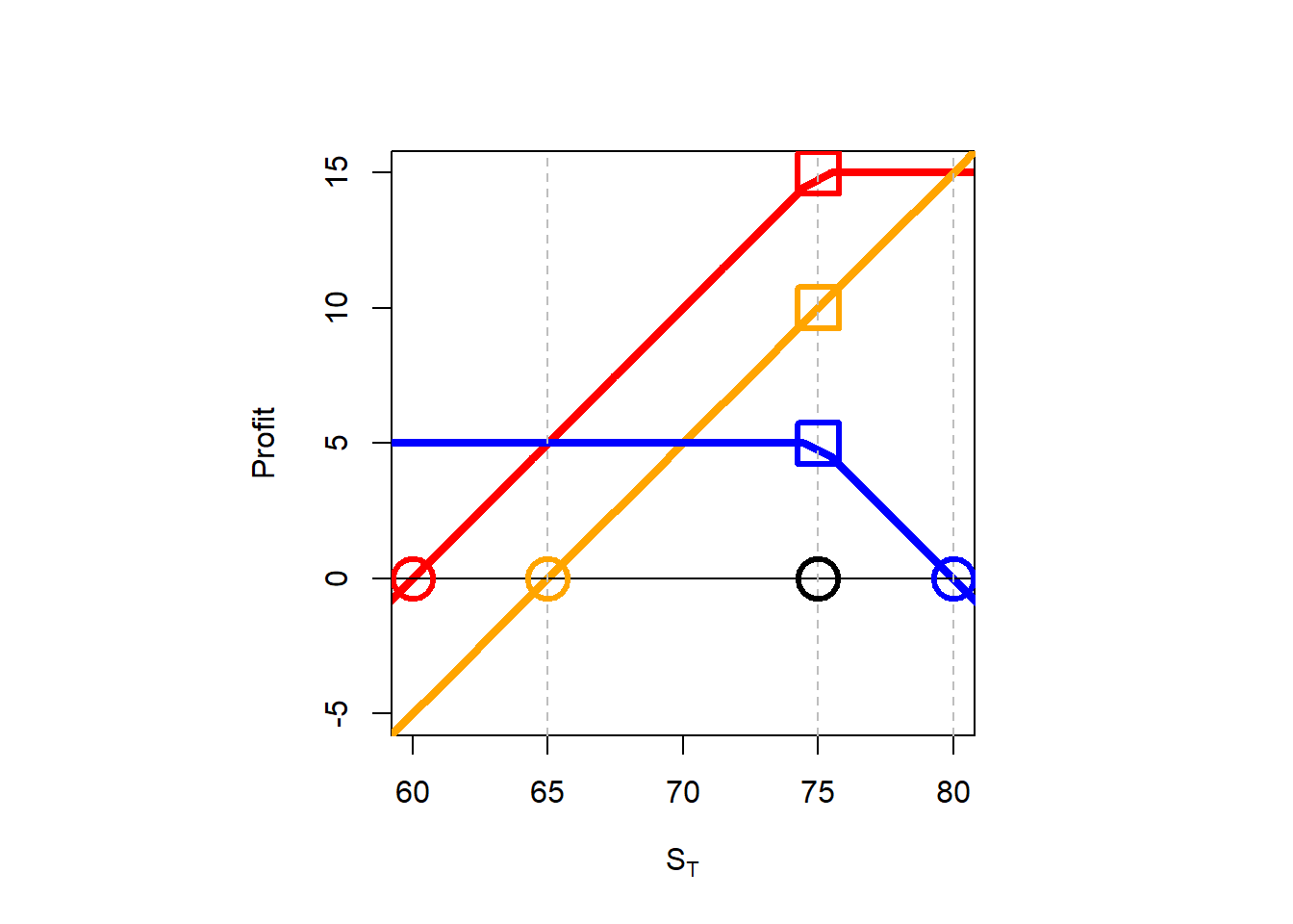
We can identify at least three isosceles right triangles, they have two sides of equal measure. The short call profit is zero at \(S_T = \$80\), in the code above: K + c_price. The stock profit is zero at \(S_T=\$65\), in the coded above: S0. Finally, the short put profit is zero at \(S_T=\$60\), in the code above: S0 - c_price.
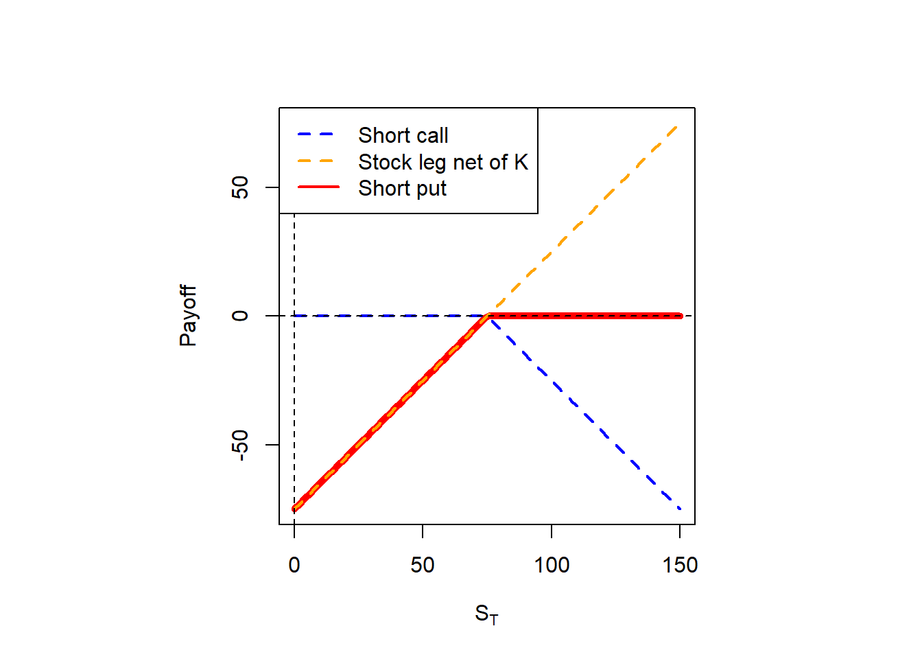
Now see how it looks if we plot a terminal payoff diagram with \(S_0=K\).
Code
S0 = K
Sl <- ST.seq - S0
cs.pr <- pmin(K - ST.seq, 0)
# A short put payoff is replicated by taking a short call and a stock leg net of K.
ans <- cs.pr + Sl
par(pty = "s")
plot(ST.seq, ans, type = "l", ylim = c(-75, 75), lwd = 5, col = "red",
     xlab = expression(paste(S[T])),
     ylab = "Payoff")
lines(ST.seq, Sl, lty = 2, lwd = 2, col = "orange")
lines(ST.seq, cs.pr, lty = 2, lwd = 2, col = "blue")
abline(v = 0, lty = 2)
abline(h = 0, lty = 2)
legend("topleft", legend = c("Short call", "Stock leg net of K", "Short put"),
       col = c("blue", "orange", "red"), lty = c(2, 2, 1),
       lwd = 2, bg = "white")