Financial options are one of the most flexible, popular and versatile financial instruments. They are relevant by themselves and important as building blocks to create other financial products and financial strategies. In order to fully understand options we need to understand their properties first. This is, what are the determinant of financial options, how these determinants change the option prices, what are the limits of financial options, what happens when these limits are violated, methods for determining the theoretical option prices and the relationship between call and put options. This section is based in Hull (2015) chapter 11.
2.1 Determinants
The main determinants of option prices are those parameters of the Black-Scholes formula under the non-dividend-paying stock assumption:
The price of the underlying stock at time zero: \(S_0\).
The option strike price: \(K\).
The risk-free rate: \(rf\).
The option maturity: \(T\).
The volatility of the underlying stock \(\sigma\).
For dividend-paying stocks, the dividend yield or income paid by the underlying asset becomes an additional determinant. Under the non-dividend-paying assumption, \(BS = f(S_0, K, rf, T, \sigma)\). Here we set up the BS function and then evaluate it at \(BS = f(S_0=50, K=50, rf=0.05, T=1, \sigma=0.3)\).
Now, let’s see how Black-Scholes option prices changes (call and put) when we leave \(S_0\) as a variable and the rest of the parameters as fixed: \(BS = f(S_0, K=50, rf=0.05, T=1, \sigma=0.3)\).
Code
# Parameters.K <-50rf <-0.05TT <-1sigma <-0.3S0 <-50# Sequence of S0.S0.seq <-seq(from =0, to =100, length.out =50)# Evaluation of the c.bs and p.bs function.c.S0 <-mapply(c.bs, S0.seq, K, rf, TT, sigma)p.S0 <-mapply(p.bs, S0.seq, K, rf, TT, sigma)
We produce as many c.S0 as values for S0.seq. Then, we can plot.
Code
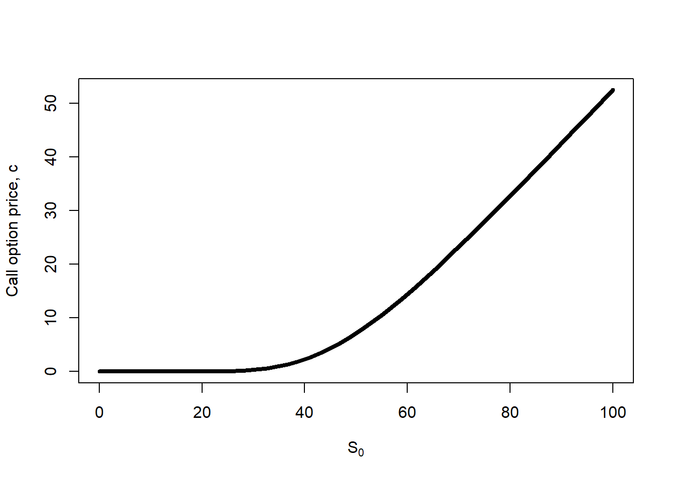
# See the results.plot(S0.seq, c.S0, type ="l", lwd =4, xlab =expression(paste(S[0])), ylab ="Call option price, c")
Figure 2.1: Call price as a function of \(S_0\).
The call option price is an increasing function of \(S_0\). This makes sense because a right to buy the stock at a fix price in the future becomes more valuable as the current value of the stock increases. In other words, it is more expensive to lock the price of an expensive asset for a potential buyer.
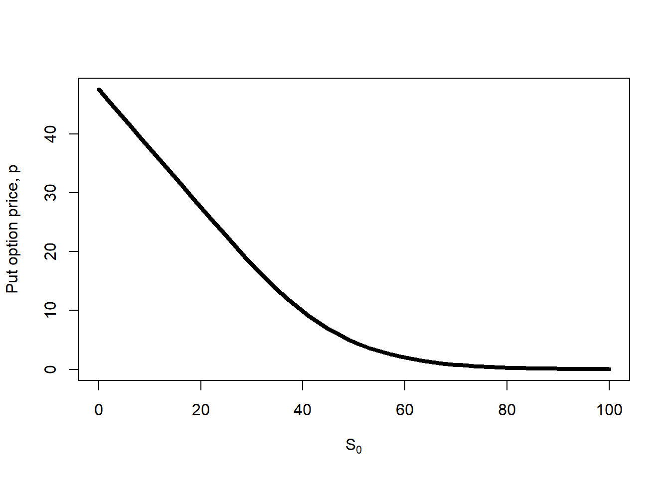
Here, it is cheaper to lock the price of an expensive asset for a potential seller. This makes sense because it looks unnecessary to lock the selling price of an expensive stock.
Let’s put both plots together.
Code
# What is the interpretation of S0.star, and how did I found this value?S0.star <- K *exp(-rf * TT)c.S0.star <-mapply(c.bs, S0.star, K, rf, TT, sigma)# Plot.plot(S0.seq, c.S0, type ="l", lwd =4, col ="blue", ylim =c(4, 8), xlab =expression(paste(S[0])), ylab ="Option theoretical price", xlim =c(40, 55))lines(S0.seq, p.S0, lwd =4, col ="red")abline(v = S0.star, lty =2)abline(h = c.S0.star, lty =2)abline(h = c, lty =2, col ="blue")abline(h = p, lty =2, col ="red")abline(v = S0, lty =2)points(S0, c, pch =19, col ="blue", cex =3)points(S0, p, pch =19, col ="red", cex =3)points(S0.star, c.S0.star, pch =19, cex =3)legend("topleft", legend =c("Call", "Put"),col =c("blue", "red"), lwd =3, bg ="white")
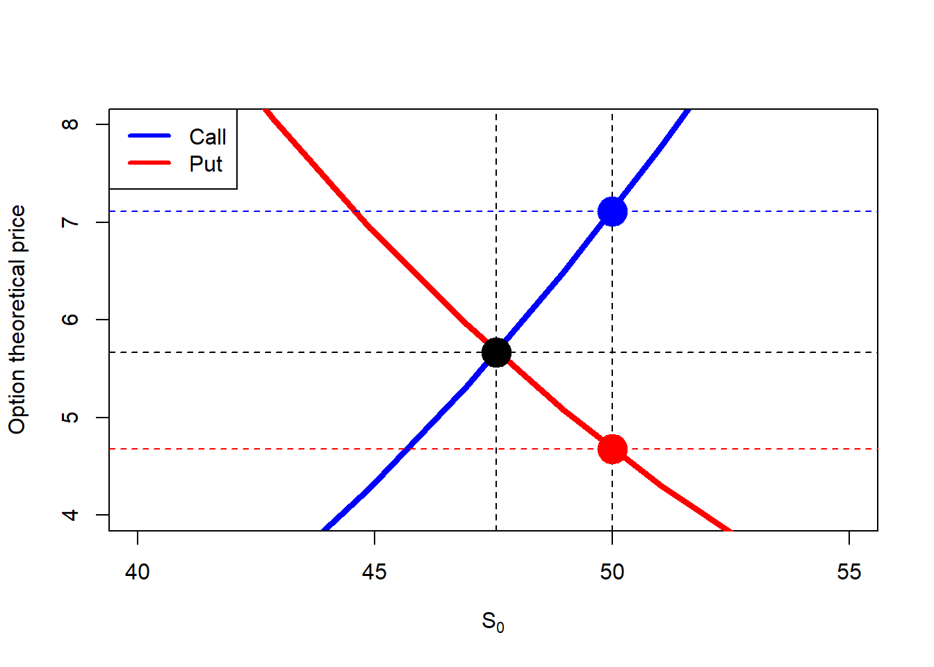
Figure 2.3: Call and put prices as a function of \(S_0\) (zoom).
Note that there is a single case in which both options (call and put) are the same. It is interesting to find out the value of \(S_0\) that makes \(c=p\). Clearly, this value is lower than \(S_0=\$50\), the point here is to find the mathematical expression of \(S_0\) that makes \(c=p\).
2.2 Option bounds
Option values (or prices) are subject or constrained to upper and lower bounds. This basically mean that in theory option prices cannot exceed upper bounds and cannot decrease below lower bounds. If they do, then arbitrage opportunities arise.
We can extend our analysis by incorporating the corresponding call and put option bounds.
Code
# Put lower bound.lb.put <-pmax(K *exp(-rf * TT) - S0.seq, 0)# Call lower bound.lb.call <-pmax(S0.seq - K *exp(-rf * TT), 0)# Again the S0.star. Where did this value comes from?line.star <- S0.star *2# Plot.par(pty ="s")plot(S0.seq, c.S0, type ="l", lwd =3, col ="blue", ylim =c(0, 100),xlab =expression(paste(S[0])), ylab ="Call (blue), put (red)")lines(S0.seq, p.S0, lwd =3, col ="red")abline(v = S0.star, lty =2) abline(v =0, lty =2)abline(v = line.star, lty =2, col ="green")abline(h = line.star, lty =2, col ="green")# Put upper bound.abline(h = K *exp(-rf * TT), lwd =2, col ="red", lty =2)lines(S0.seq, lb.put, lwd =2, col ="red", lty =2)# Call upper bound.lines(S0.seq, S0.seq, lwd =2, col ="blue", lty =2) lines(S0.seq, lb.call, lwd =2, col ="blue", lty =2)
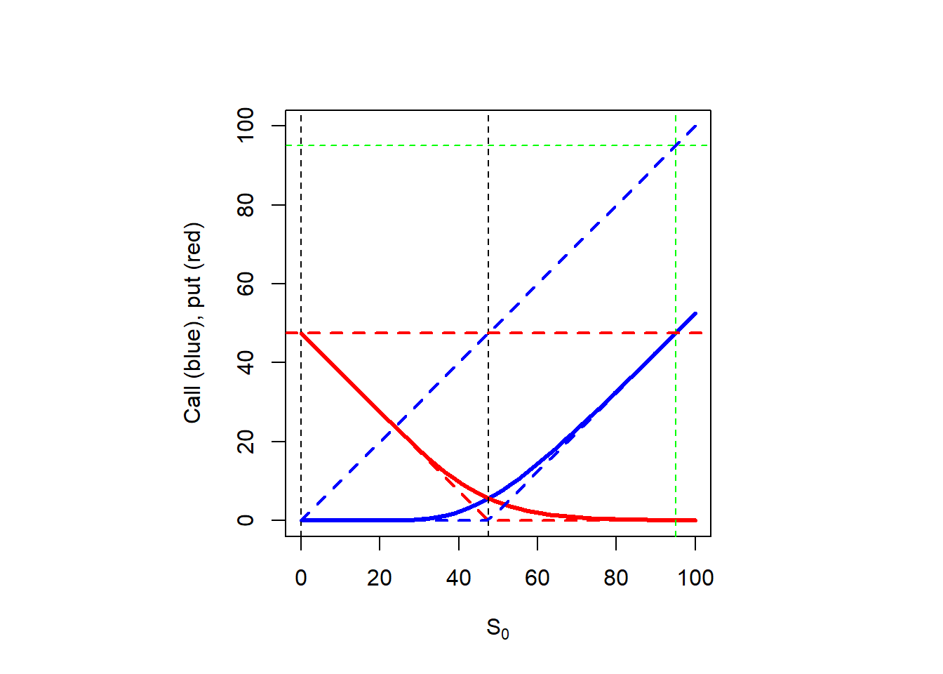
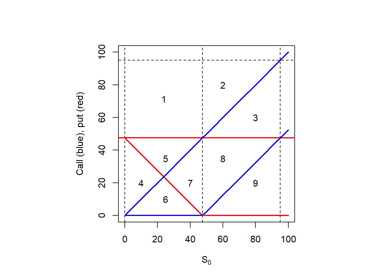
Figure 2.4: Option values as a function of \(S_0\) including option bounds.
Note that the stock price range of values is from zero to positive infinity. However, this is not the case for the options. The option values depend on these bounds. We can illustrate the same plot in a cleaner way, to make emphasis on a geometric approach.
Figure 2.5: Call and put option bounds: geometric inspection (or ‘the puzzle’).
Every number from 1 to 9 is assigned to a specific geometric shape in the plot above. This is, a square as in 1, and triangles of two different shapes in the rest of the cases (2 to 9). It is interesting to analyze whether each area represents a possible price range for call and/or put options.
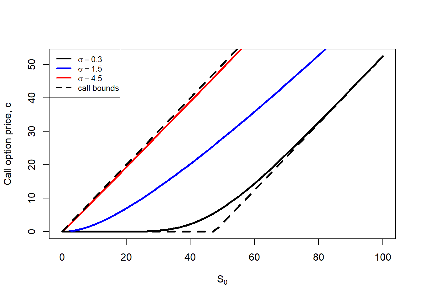
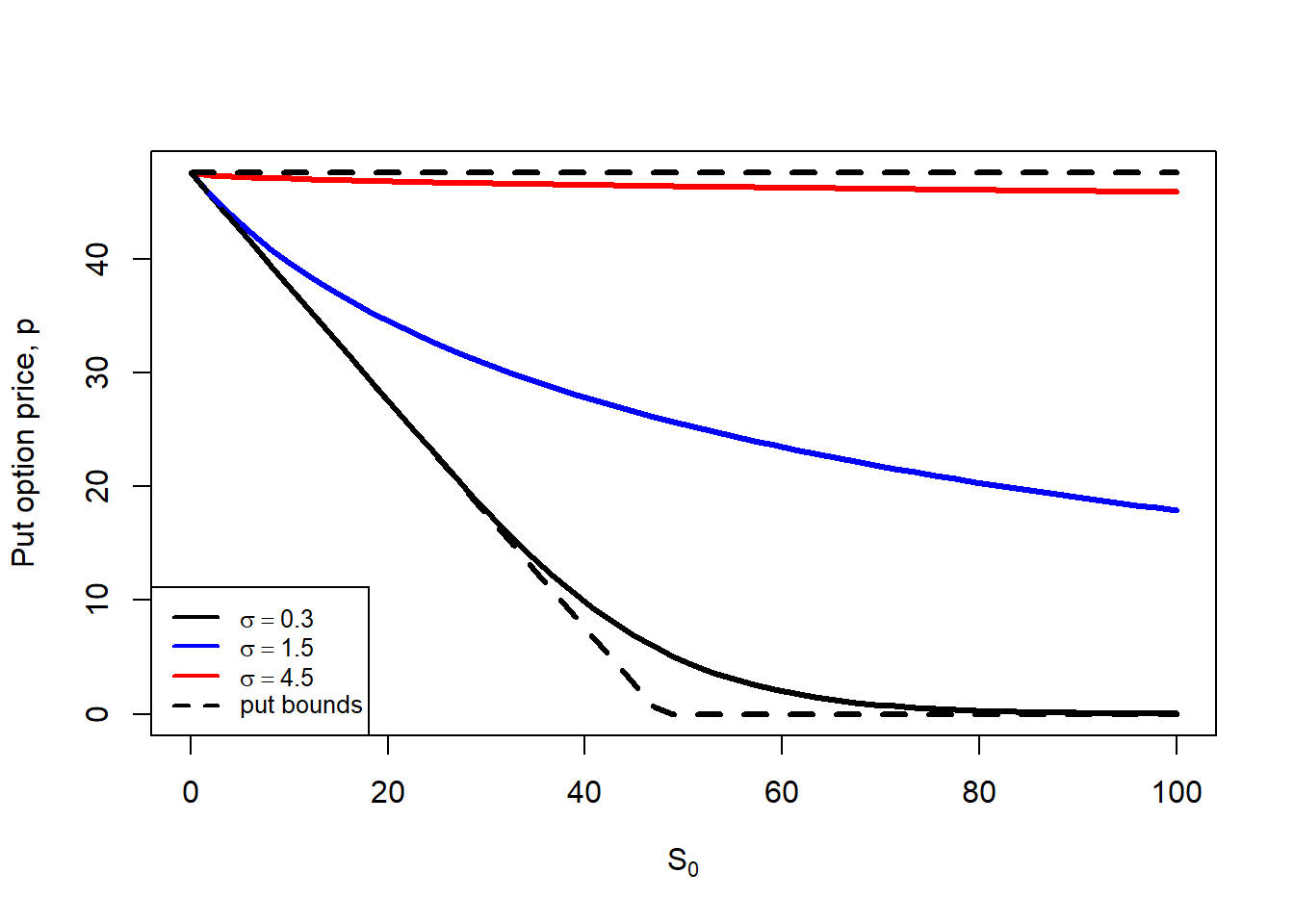
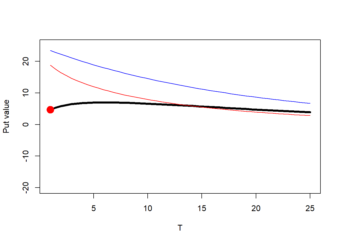
Now, let’s see how Black-Scholes option prices changes (call and put) when we leave \(S_0\) as a variable, three levels of \(\sigma\) and the rest of the parameters as fixed: \(BS = f(S_0, K=50, rf=0.05, T=1, \sigma)\). We can show this in a 2 dimension plot, including the correspondent bounds.
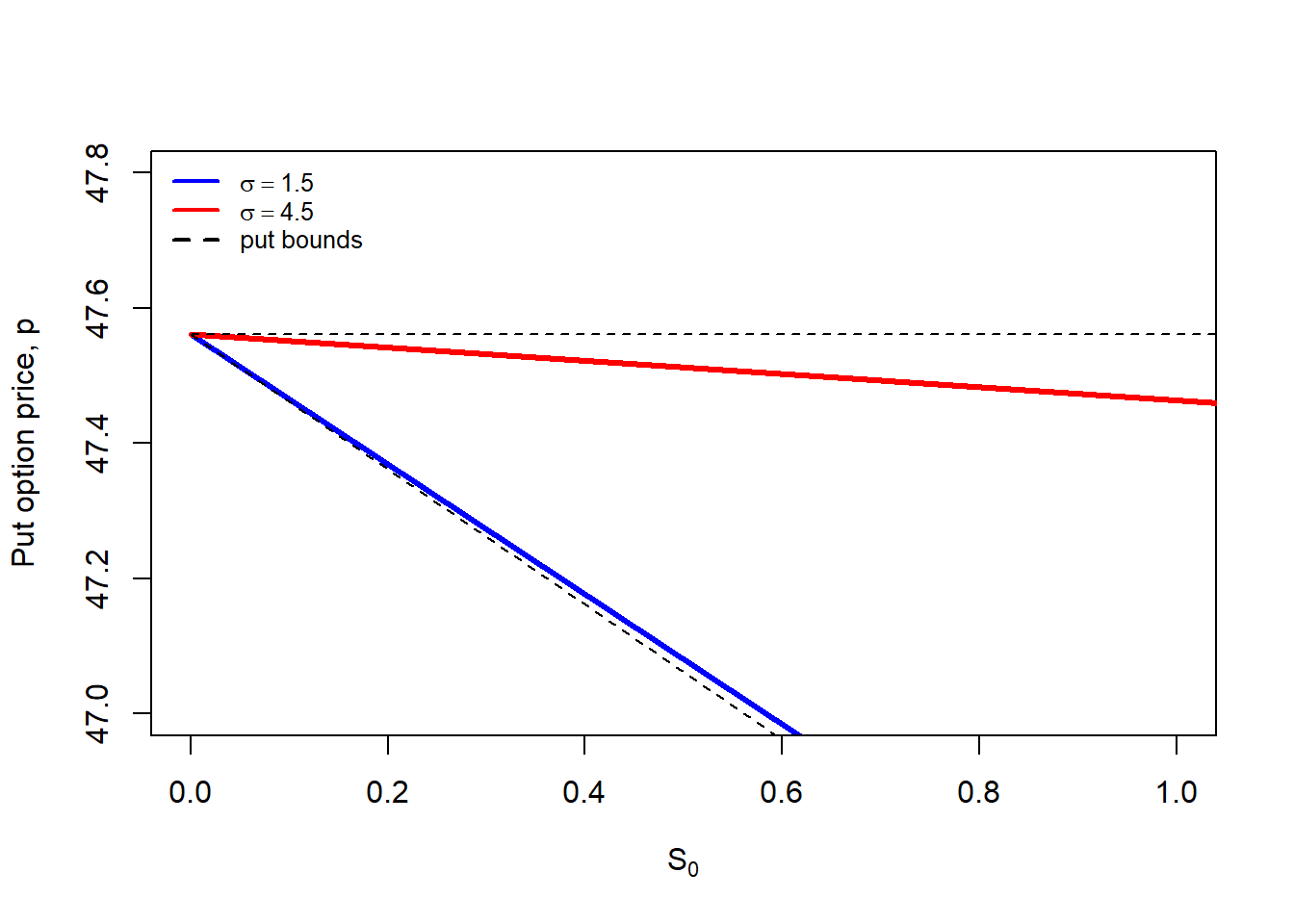
Figure 2.8: Put option changes as \(S_0\) and \(\sigma\) increase: the role of bounds (zoom).
Then, regardless of the extreme value of parameters, option bounds represent the maximum and minimum values for the call and put options. These option prices are theoretical as they are calculated by implementing the Black-Scholes formula. We normally evaluate whether the option market prices violates these bounds because this will flag an opportunity to implement an arbitrage strategy to generate a risk-free profit.
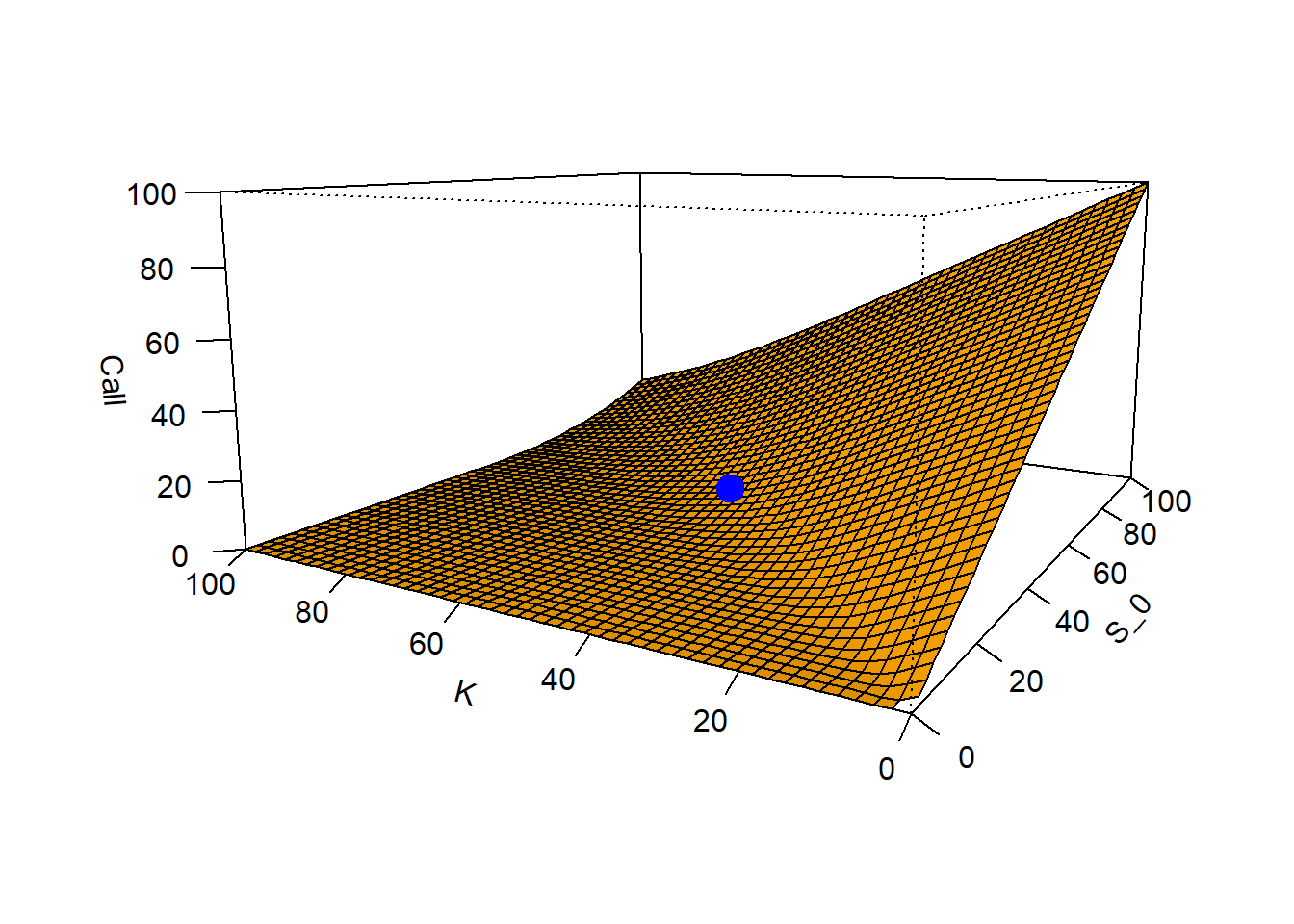
A different way to illustrate the option properties is by looking at a plane. Here, we let \(S_0\) and \(K\) as a free variables and remain the rest as fixed: \(BS = f(S_0, K, rf=0.05, T=1, \sigma = 0.3)\).
Code
# K as a variable.K.seq <- S0.seq# Create the empty matrix.c.S0.s <-matrix(0, nrow =50, ncol =50)# Fill the empty matrix.for(i in1:50){ # Is there an easier way to do this?for(j in1:50){ c.S0.s[i, j] <-c.bs(S0.seq[i], K.seq[j], rf, TT, sigma) } }# Plot.c.S0.s.plot <-persp(S0.seq, K.seq, c.S0.s, zlab ="Call", xlab ="S_0", ylab ="K", theta =-60, phi =10, expand =0.5, col ="orange", shade =0.2, ticktype ="detailed") points(trans3d(S0, K, c, c.S0.s.plot), cex =2, pch =19, col ="blue")
Figure 2.9: Call value as \(S_0\) and \(K\) change, a plane view.
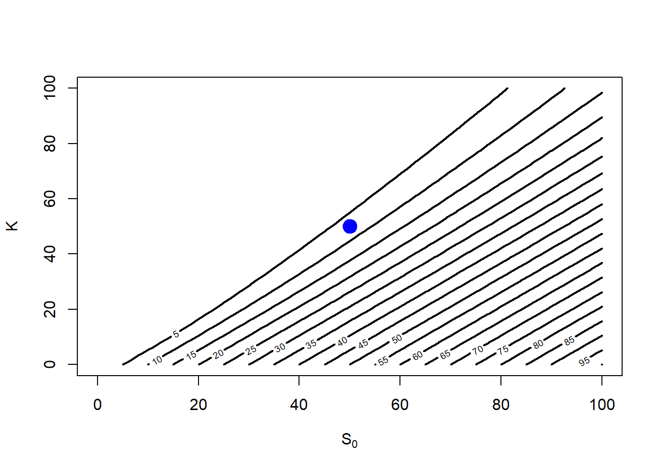
An alternative view is by showing a contour plot. A contour plot is a graphical technique for representing a 3-dimensional surface by plotting constant \(z\) slices (option prices), called contours, on a 2-dimensional format. That is, given a value for \(z\), lines are drawn for connecting the \((x, y)\) coordinates (\(S_0\), \(K\)) where that \(z\) value occurs.
Figure 2.10: Call value as \(S_0\) and \(K\) change, a contour view.
Note that the blue circle \(S_0=\$50, K=\$50\) is between the contour line 5 and 10, this makes sense because the call option at \(call(S_0=50, K=50, rf=0.05, T=1, \sigma = 0.3) = \$7.115627\).
Code
plot_ly(type ="surface" , x = S0.seq, y = K.seq , z = c.S0.s ) %>%layout(scene =list(xaxis =list(title ="Stock price"), yaxis =list(title ="K", zaxis =list(title ="Call price")))) %>%hide_colorbar()
Figure 2.11: Call value as \(S_0\) and \(K\) change, an interactive view.
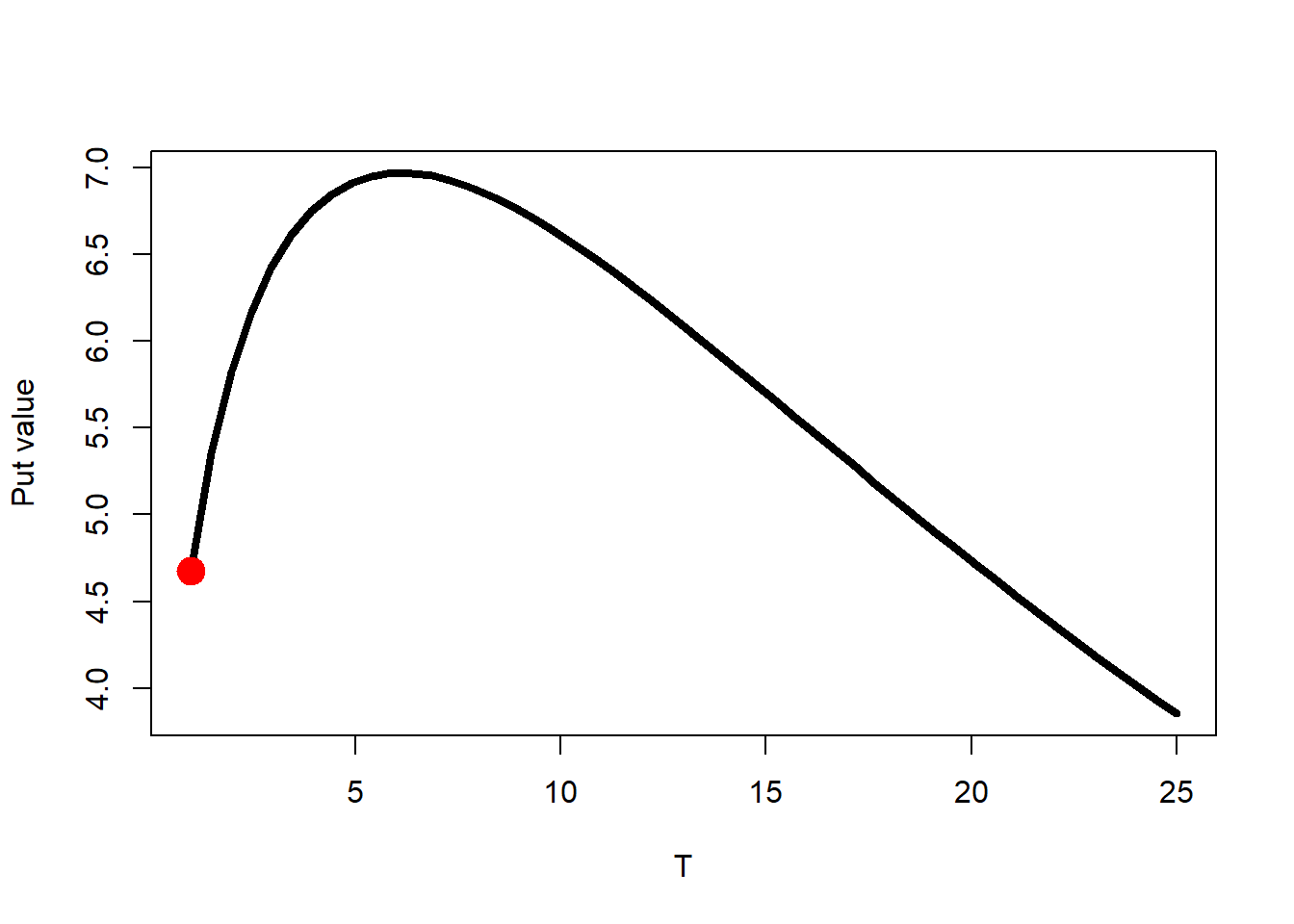
An interesting case is the value of the put as a function of the time to maturity. Let’s see the simplest case.
Code
TT.seq <-seq(from =1, to =25, length.out =50)p.TT <-mapply(p.bs, S0, K, rf, TT.seq, sigma)plot(TT.seq, p.TT, type ="l", lwd =4, ylab ="Put value", xlab ="T")points(TT, p, col ="red", cex =2, pch =19)
Figure 2.12: European put as \(T\) increases: the mysterious hump.
The put option price first increases as the time to maturity increases and after reaching a maximum, the put option price decreases. What is the mathematical expression for the time to maturity which makes the put option price maximum? What is the reason or logic behind this mysterious hump? Those are interesting questions to address.
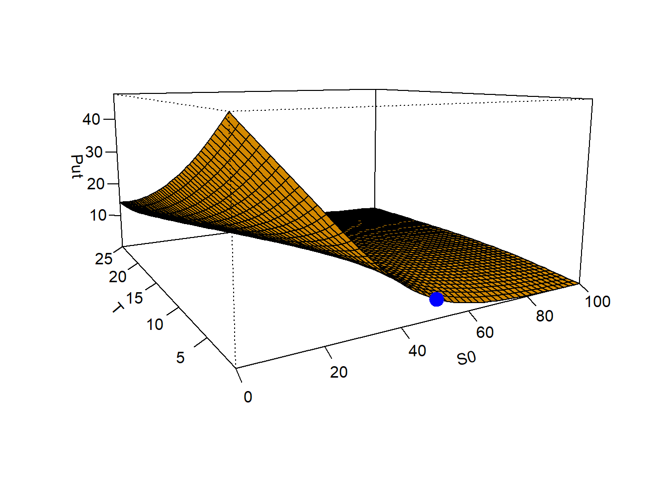
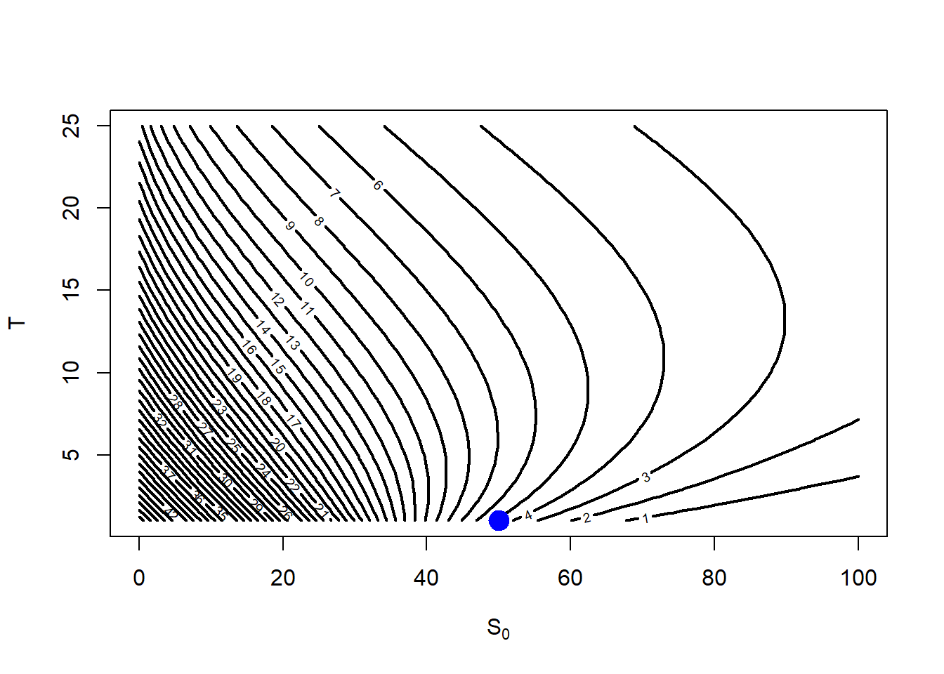
Figure 2.14: Put value as \(S_0\) and \(T\) change, a contour view, or the hypnotic plot.
Now the mysterious hump is clearer than before. Remember the value of \(put(S_0=50, K=50, rf=0.05, T=1, \sigma = 0.3) = \$4.677099\).
Code
plot_ly(type ="surface" , x = S0.seq, y = TT.seq , z = p.S0.T ) %>%layout(scene =list(xaxis =list(title ="Stock price"), yaxis =list(title ="T", zaxis =list(title ="Put price")))) %>%hide_colorbar()
Figure 2.15: Put value as \(S_0\) and \(T\) change, an interactive view.
2.3 Put-call parity
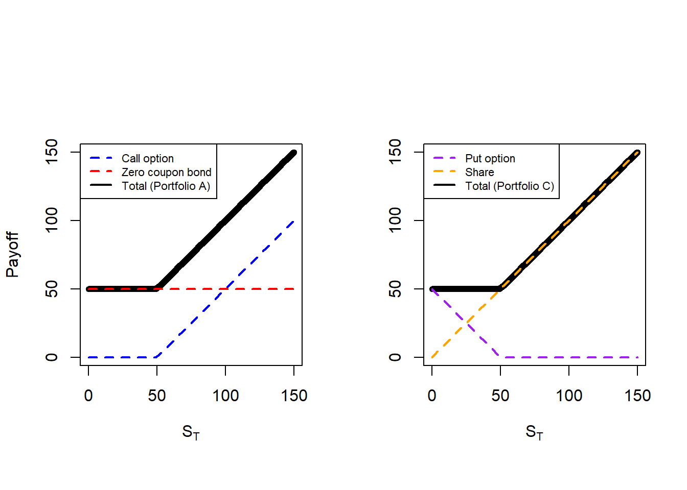
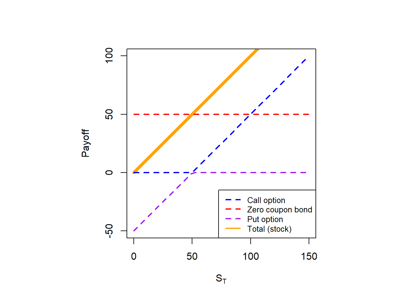
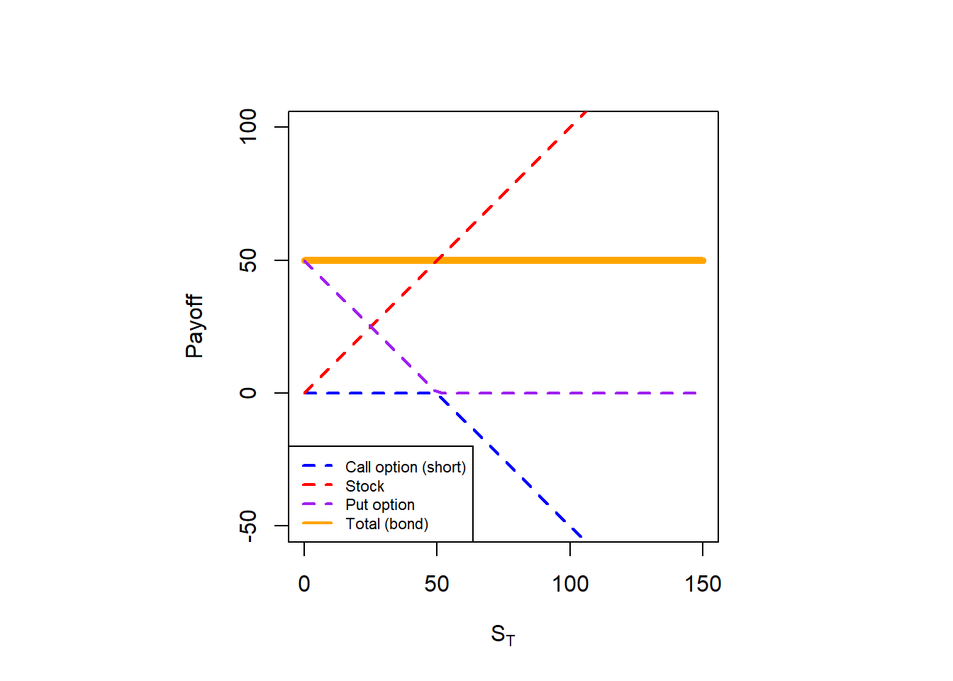
The main idea behind the put-call parity is to understand how call and put option prices are related as today, at \(t=0\). In Hull, the procedure to derive the put-call parity starts with the definition of two portfolios: (1) a call and a bond; (2) a put and a stock. Then, derive the corresponding payoff of each portfolio at maturity. Doing this is relatively easy because we do not need a valuation method as we know the payoff functions for options, bonds and stocks. Given that we can demonstrate that the value of two different portfolios are the same at \(T\), then we can conclude that these two portfolios are worth the same at \(t=0\) as well.
Figure 2.16: Portfolio A and C payoffs, the put-call parity.
The point here is that the black line (total) is the same in both cases. This is why we argue that the payoffs of both portfolios are worth the same. If this is so, then they are worth the same in time \(t=0\).
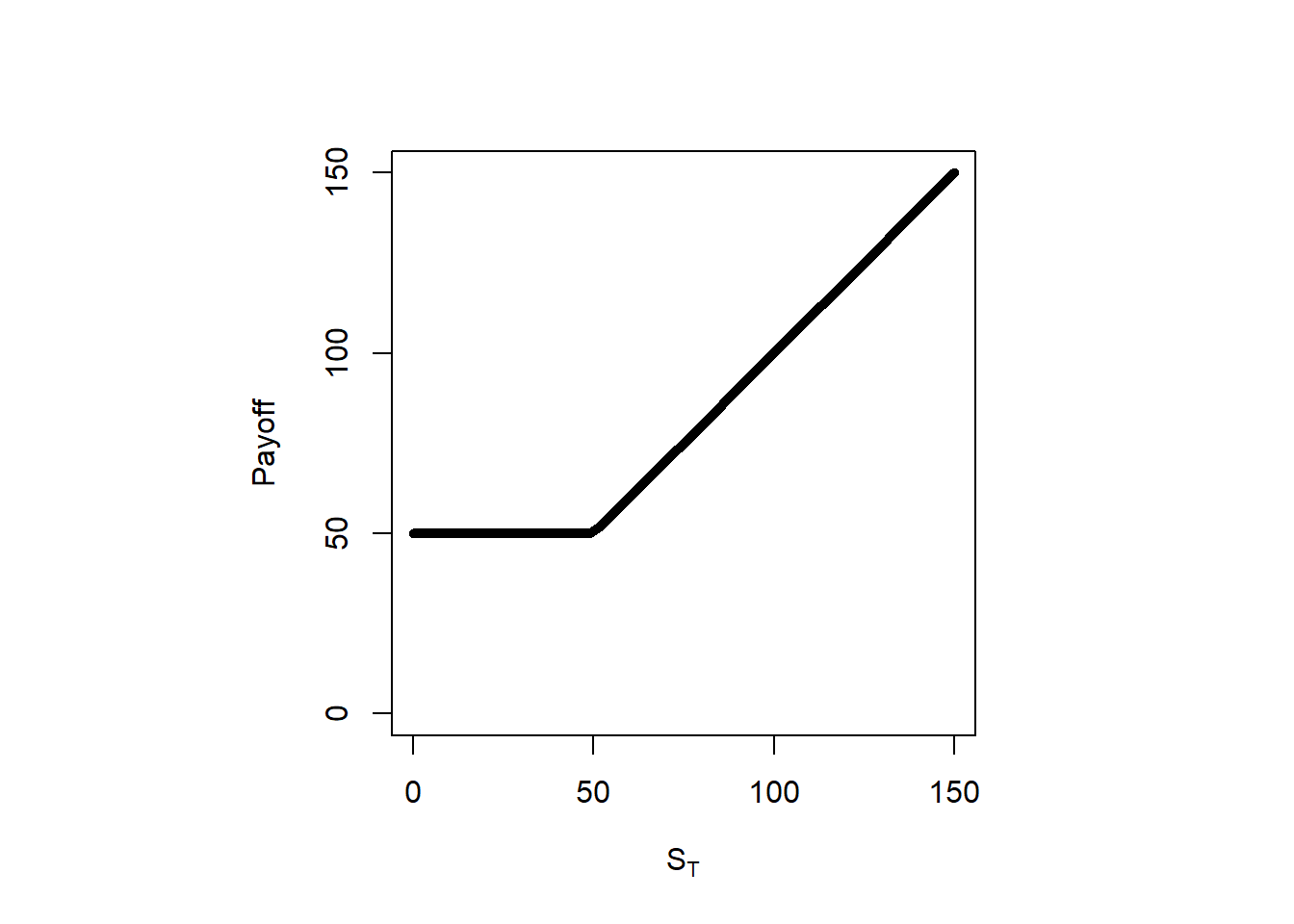
In sum, this is the payoff of portfolios A and C: \(\mathrm{max}(S_T,K)\). This is already stored in pc.
So, we created a stock that did not exist with a call, a bond and a put. We can manipulate the put-call parity to create a synthetic bond \(Ke^{-rT}\). This is:
There is an alternative to the Black-Scholes formula we indirectly review before. Next section introduces the binomial trees.
2.4 Binomial trees
Binomial trees are a flexible valuation method for options because we can use them to value not only European but also American options. This section is based in Hull (2015) chapter 13.
We can evaluate the function above to see how the price change depending on the number of steps in the binomial tree. Let’s evaluate the bin() function assuming \(S_0=\$50\), \(K=\$50\), \(rf=0.05\), \(T=1\), and \(\sigma=0.3\) at different time steps.
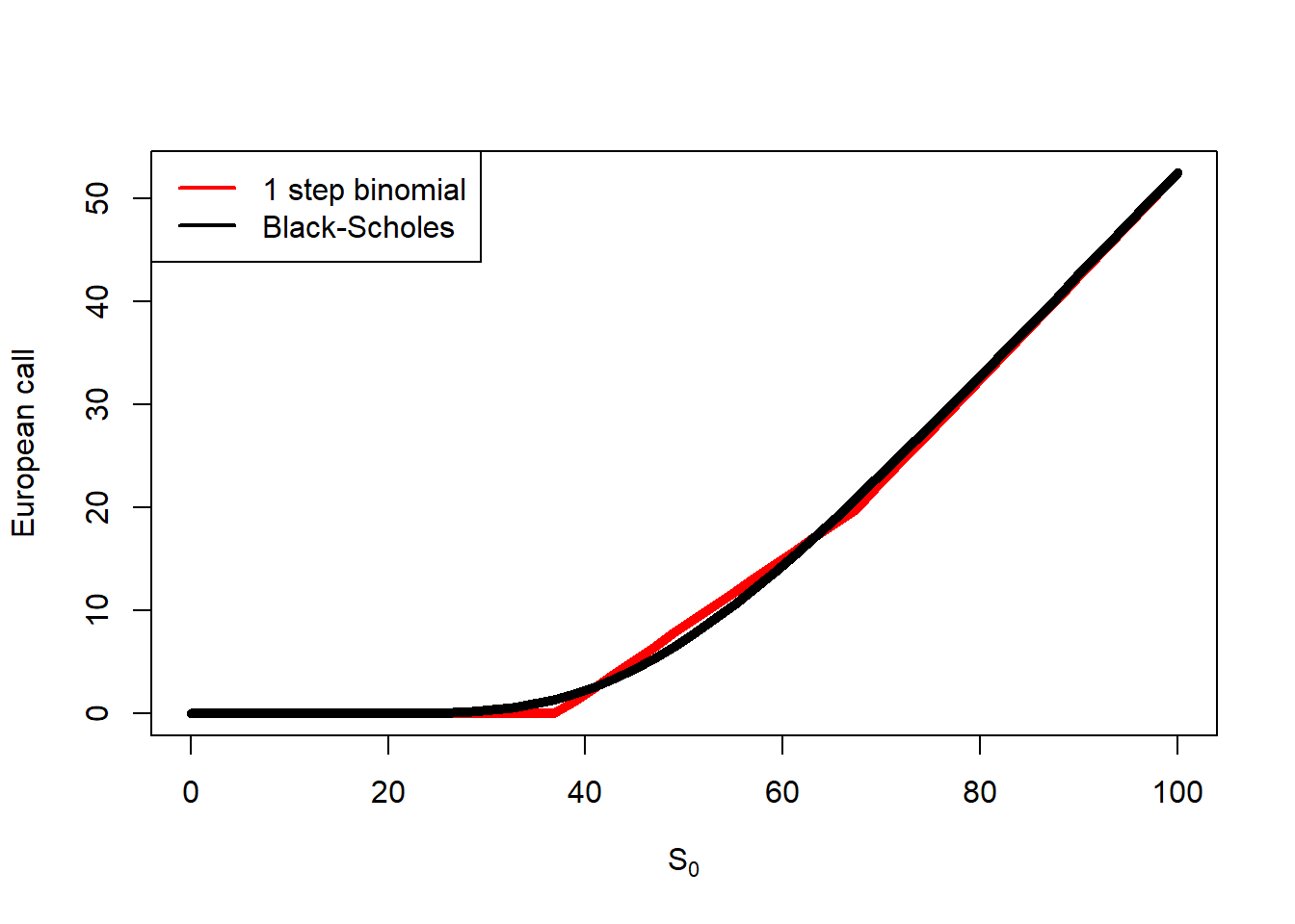
Here, we compare the value of the binomial method and the Black-Scholes at different time steps as a function of \(S_0\).
Code
plot(S0.seq, b1[1, ], type ="l", col ="red", lwd =5, xlab =expression(paste(S[0])), ylab ="European call")lines(S0.seq, c.S0.s1, col ="black", lwd =5)legend("topleft", legend =c("1 step binomial", "Black-Scholes"),col =c("red", "black"), lwd =2, bg ="white")
Figure 2.20: One-step binomial and Black-Scholes comparison.
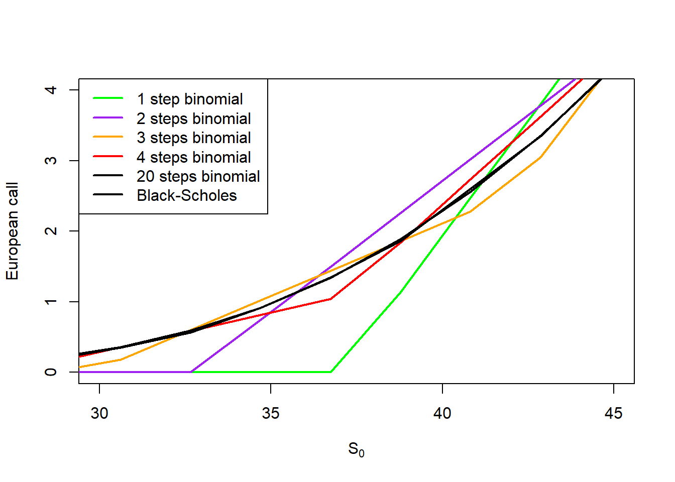
There are some differences between the binomial and the Black-Scholes. Let’s zoom to see the differences clearer.
Code
plot(S0.seq, b1[1,], type ="l", ylim =c(0, 4), xlim =c(30, 45), col ="green", lwd =2, xlab =expression(paste(S[0])), ylab ="European call")lines(S0.seq, b2[1,], col ="purple", lwd =2)lines(S0.seq, b3[1,], col ="orange", lwd =2)lines(S0.seq, b4[1,], col ="red", lwd =2)lines(S0.seq, b20[1,], col ="black", lwd =2)lines(S0.seq, c.S0.s1, col ="black", lwd =2)legend("topleft", legend =c("1 step binomial", "2 steps binomial", "3 steps binomial", "4 steps binomial","20 steps binomial", "Black-Scholes"),col =c("green", "purple", "orange", "red", "black", "black"), lwd =2, bg ="white")
Figure 2.21: Binomial and Black-Scholes convergence, a zoom view.
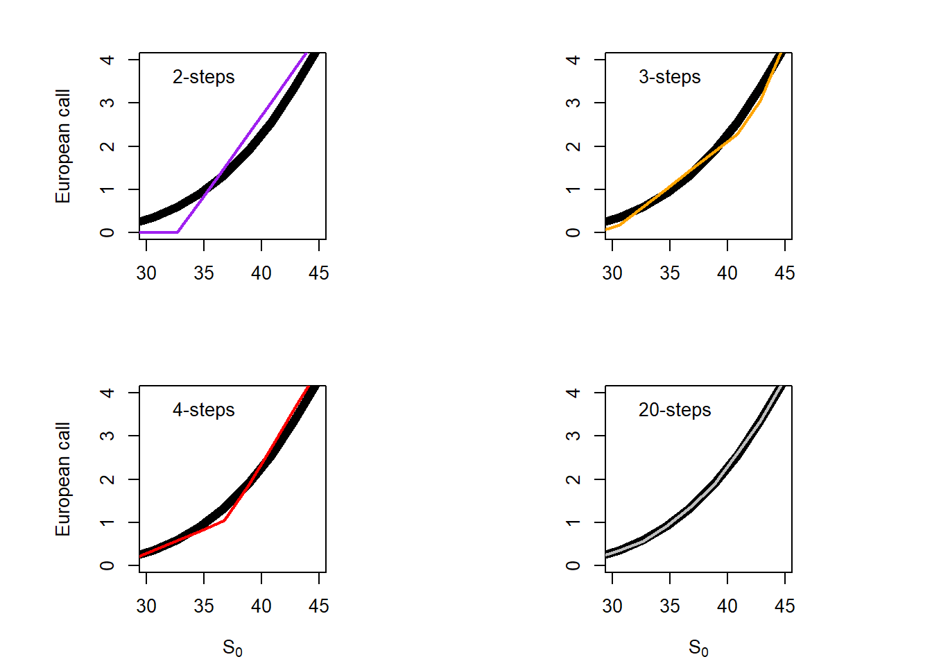
Not clear yet. Let’s see a panel view.
Code
par(mfrow =c(2, 2), mai =c(0.7, 0.4, 0.4, 0.4))par(pty ="s")plot(S0.seq, c.S0.s1, type ="l", ylim =c(0, 4), xlim =c(30, 45), col ="black", lwd =6, xlab ="", ylab ="European call")lines(S0.seq, b2[1,], col ="purple", lwd =2)legend("topleft", legend =c("2-steps"),bg ="white", bty ="n")par(pty ="s")plot(S0.seq, c.S0.s1, type ="l", ylim =c(0, 4), xlim =c(30, 45), col ="black", lwd =6, xlab ="", ylab ="")lines(S0.seq, b3[1,], col ="orange", lwd =2)legend("topleft", legend =c("3-steps"),bg ="white", bty ="n")par(pty ="s")plot(S0.seq, c.S0.s1, type ="l", ylim =c(0, 4), xlim =c(30, 45), col ="black", lwd =6, xlab =expression(paste(S[0])), ylab ="European call")lines(S0.seq, b4[1,], col ="red", lwd =2)legend("topleft", legend =c("4-steps"), bg ="white", bty ="n")par(pty ="s")plot(S0.seq, c.S0.s1, type ="l", ylim =c(0, 4), xlim =c(30, 45), col ="black", lwd =6, xlab =expression(paste(S[0])), ylab ="")lines(S0.seq, b20[1,], col ="grey", lwd =2)legend("topleft", legend =c("20-steps"),bg ="white", bty ="n")
Figure 2.22: Binomial and Black-Scholes convergence, a panel view.
As stated above, the binomial method converges to the Black-Scholes as time steps increase. We can also create a function to visualize the price path of the stock from \(S_0\) to \(S_T\) given the assumptions of the binomial method.
2.6 Stock price paths
In order to value option prices, we first need to understand the evolution of the underlying (in this case the stock price) from time zero to maturity, this is from \(S_0\) to \(S_T\). The binomial method assumes that the price can increase or decrease with a certain probability in each time step. Here, we can show how the binomial tree method assumes this stock price evolution.
Let’s assume 10-steps, from \(t=0.1, t=0.2,..., t=1\)
Code
# Function to generate stock prices paths given the binomial method.S.paths <-function(S0, sigma, TM, steps) { dt <- TM / steps u <-exp(sigma * dt^0.5) # Here we set u and d as a function of sigma. d <-exp(-sigma * dt^0.5) S <-matrix(0, (steps +1), (steps +1)) S[1, 1] <- S0for(i in2:(steps +1)) { do =seq(0, i -1) up =rev(do) # rev provides a reversed version of its argument. S[(1:i), i] = S0 * (u ^ up) * (d ^ do) } S }# Evaluate the function.Spaths <-S.paths(50, 0.3, 1, 10)# A table.colnames(Spaths) <-c(0, cumsum(rep(1/10, 10)))round(Spaths, 2)
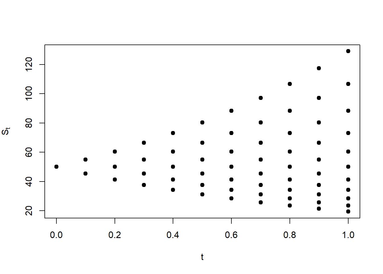
This does not look like a typical binomial tree. In fact, it is not very clear whether a given price corresponds to an increase or decrease from a previous time step. We can make a few arrangements to visualize this as a tree.
Code
S.paths <-function(S0, sigma, TM, steps) { dt <- TM / steps u <-exp(sigma * dt^0.5) d <-exp(-sigma * dt^0.5) S <-matrix(0, 2* ((steps +1)), (steps +1)) S2 <-matrix(NA, ((2* steps) +2), (steps +1)) S2[(steps +1), 1] <- S0for(i in2:(steps +1)) { do =seq(0, i -1) up =rev(do) # rev provides a reversed version of its argument. S[(1:i), i] = S0 * (u ^ up) * (d ^ do) x =rep(NA, i) # These are the NA between stock prices. r =rev(c(seq(0, (steps -1)), 0)) # These creates the blank spaces.# Here we combine NA and stock prices for each column. S2[(1+ r[i]):((2* i) + r[i]), i] =as.numeric(rbind(S[(1:i), i], x)) } S2 }# Evaluate the function.Spaths <-S.paths(50, 0.3, 1, 10)# A table.colnames(Spaths) <-round(c(0, cumsum(rep(1/10, 10))), 2)round(Spaths, 2)
       0   0.1   0.2   0.3   0.4   0.5   0.6   0.7    0.8    0.9      1
 [1,] NA    NA    NA    NA    NA    NA    NA    NA     NA     NA 129.12
 [2,] NA    NA    NA    NA    NA    NA    NA    NA     NA 117.43     NA
 [3,] NA    NA    NA    NA    NA    NA    NA    NA 106.80     NA 106.80
 [4,] NA    NA    NA    NA    NA    NA    NA 97.13     NA  97.13     NA
 [5,] NA    NA    NA    NA    NA    NA 88.34    NA  88.34     NA  88.34
 [6,] NA    NA    NA    NA    NA 80.35    NA 80.35     NA  80.35     NA
 [7,] NA    NA    NA    NA 73.08    NA 73.08    NA  73.08     NA  73.08
 [8,] NA    NA    NA 66.46    NA 66.46    NA 66.46     NA  66.46     NA
 [9,] NA    NA 60.45    NA 60.45    NA 60.45    NA  60.45     NA  60.45
[10,] NA 54.98    NA 54.98    NA 54.98    NA 54.98     NA  54.98     NA
[11,] 50    NA 50.00    NA 50.00    NA 50.00    NA  50.00     NA  50.00
[12,] NA 45.47    NA 45.47    NA 45.47    NA 45.47     NA  45.47     NA
[13,] NA    NA 41.36    NA 41.36    NA 41.36    NA  41.36     NA  41.36
[14,] NA    NA    NA 37.62    NA 37.62    NA 37.62     NA  37.62     NA
[15,] NA    NA    NA    NA 34.21    NA 34.21    NA  34.21     NA  34.21
[16,] NA    NA    NA    NA    NA 31.11    NA 31.11     NA  31.11     NA
[17,] NA    NA    NA    NA    NA    NA 28.30    NA  28.30     NA  28.30
[18,] NA    NA    NA    NA    NA    NA    NA 25.74     NA  25.74     NA
[19,] NA    NA    NA    NA    NA    NA    NA    NA  23.41     NA  23.41
[20,] NA    NA    NA    NA    NA    NA    NA    NA     NA  21.29     NA
[21,] NA    NA    NA    NA    NA    NA    NA    NA     NA     NA  19.36
[22,] NA    NA    NA    NA    NA    NA    NA    NA     NA     NA     NA
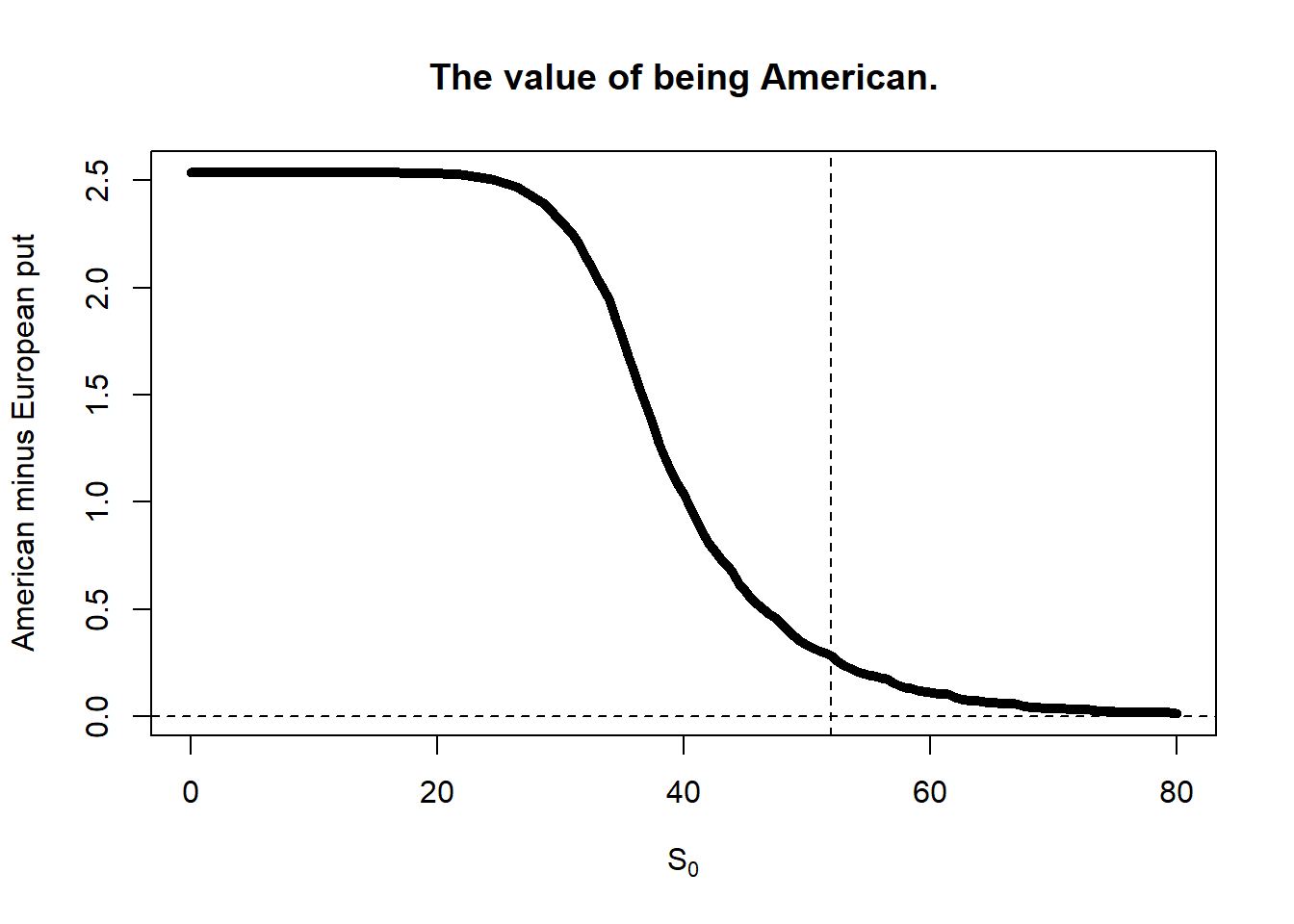
There is no difference between American and European call options theoretical prices for non-dividend-paying stocks, because there are no incentives to exercise American call options early. The case of put options is different as incentives to exercise American put options early may arise. As a consequence, American put options are in general more expensive than European put options.
Let’s evaluate this difference in a 50-step case: \(K=\$52\), \(\sigma = 0.3\), \(T=2\), \(rf=0.05\), and different values of \(S_0\).
Code
S.seq <-seq(0, 80, 0.5)AEoptions <-mapply(bin, S.seq, 52, 0.3, 1, 0.05, 50)plot(S.seq, unlist(AEoptions[4,]) -unlist(AEoptions[2,]), type ="l", lwd =5, main ="The value of being American.",xlab =expression(paste(S[0])),ylab ="American minus European put")abline(v =52, lty =2)abline(h =0, lty =2)
Figure 2.24: The value of being American; or the cost of being European.
2.7 Real vs. risk-neutral world
This section is based on Hull (2015) section 13.1. A stock price is currently $20, and it is known that at the end of 3 months it will be either $22 or $18. We are interested in valuing a European call option to buy the stock for $21 in 3 months. The risk-neutral probability \(p\) for the case of \(rf=0.12\), \(T=3/12\), \(u=1.1\) and \(d=0.9\):
\(p = \frac{e^{rT}-d}{u-d} \rightarrow p = \frac{e^{0.12\times(3/12)}-0.9}{1.1-0.9} \rightarrow p = 0.6522727\).
Code
# This is the substitution of equation 13.3.rnp <- (exp(0.12*(3/12))-0.9)/(1.1-0.9)rnp
[1] 0.6522727
Following Hull (2015), this option will have one of two values at the end of the 3 months. If the stock price turns out to be $22, the value of the option will be $1; if the stock price turns out to be $18, the value of the option will be zero. This is the European call option expected value at time \(T\):
We can calculate the European call option value at \(t=0\) according to the risk-neutral valuation. This option value \(f\) is valid in the real world, not only in the risk-neutral world.
\(f = \$0.6522727 \times e^{-rT} \rightarrow f = \$0.6522727 \times e^{-0.12\times3/12} \rightarrow f = \$0.6329951\).
Code
option_0 <- option_T *exp(-0.12*(3/12))option_0
[1] 0.6329951
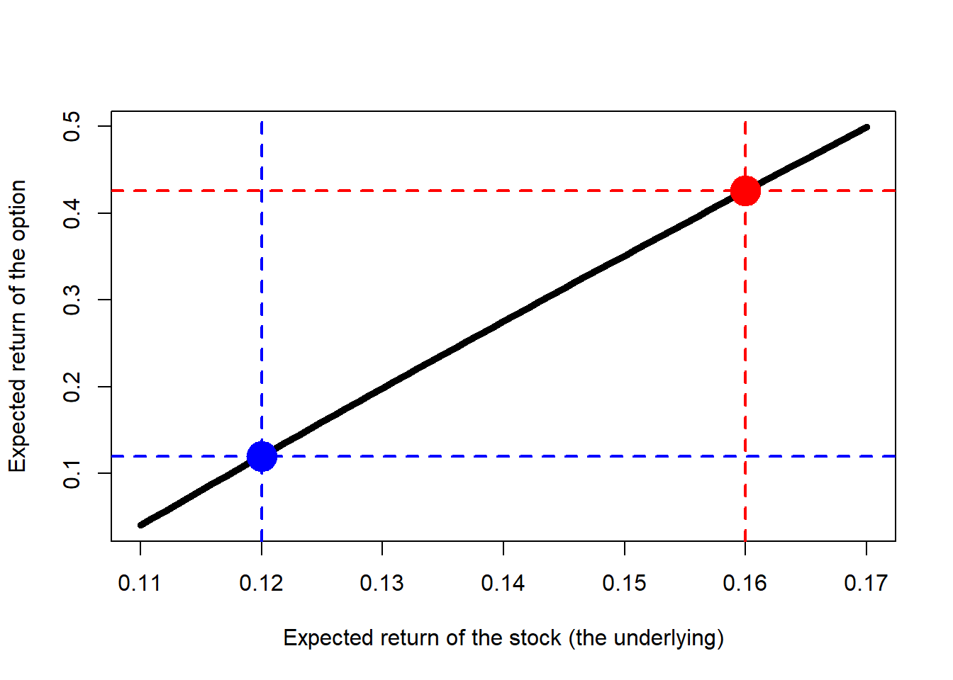
Suppose that, in the real world, we know the expected return on the stock is \(\mu=16\%\). This is easily calculated as we have historical information of stock returns. It is also a reasonable assumption as this is higher than the risk-free rate. Then, the probability of an up movement in the real world \(p^*\) is:
Can we calculate the present value of $0.7040539? We need the option discount factor in the real world. The problem is that this rate is usually unknown. In this example, the discount rate implied by the next calculation is higher than the risk-free rate and the expected return on the stock. Using risk-neutral valuation solves this problem because we know that in a risk-neutral world the expected return on all assets (and therefore the discount rate to use for all expected payoffs) is the risk-free rate.
What can we do to find out the option discount factor? Since we know the correct value of the option is \(f=\$0.6329951\) in both real and risk-neutral world, we can deduce the real-world discount rate \(r\) of this European call option.
We know this is true: \(\$0.6329951 = \$0.704053e^{-r\times3/12}\).
Then, solve for \(r\): \(\rightarrow \frac{\$0.6329951}{\$0.704053} = e^{-r\times3/12}\),
# Evaluate the function in a range of values.r.seq <-seq(0.11, 0.17, 0.001)df <-mapply(option.df.fun, r.seq)plot(r.seq, df, type ="l", lwd =5, xlab ="Expected return of the stock (the underlying)",ylab ="Expected return of the option")points(0.12, 0.12, pch =19, col ="blue", cex =3)points(0.16, 0.4255688, pch =19, col ="red", cex =3)abline(v =0.12, lty =2, col ="blue", lwd =2)abline(h =option.df.fun(0.12), lty =2, col ="blue", lwd =2)abline(v =0.16, lty =2, col ="red", lwd =2)abline(h =option.df.fun(0.16), lty =2, col ="red", lwd =2)
Figure 2.25: Red pill, blue pill.
As in the movie, The Matrix, the blue pill describes living life without knowing its meaning or running away from the truth in order to stay as is. This is equivalent to the risk-neutral world. The red pill is described as the solution for knowing the real truth in life. This is equivalent to the real-world.
2.8 Parrondo’s paradox
The Parrondo’s paradox is controversial in the literature, we are not going to elaborate on that. However, it is indeed interesting as it looks counterintuitive: Can we combine two losing investments into a winner?
This video was created by Professor Humberto Barreto from DePauw University, Indiana, based on a now-defunct app from Alexander Bogomolny of the well-known maths site Cut the Knot. It illustrates the general idea of Parrondo’s paradox.
Code
embed_url("https://youtu.be/cEuyfD2qVgQ")
Consider asset A which has a known 6% gross return. In the context of a binomial tree: \([p\times(1+u)]+[(1-p)\times(1-d)]=1.06\). Let’s assume \(p=0.5\), so we have:
\(0.5(1+u)+0.5(1-d)=1.06\).
Asset A has a known 40% volatility, so:
\(0.4=\sqrt{0.5(1+u)^2+0.5(1-d)^2-1.06^2}\).
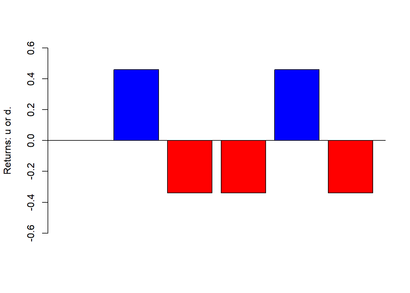
We have two equations and two unknown variables, so we can solve for \((1+u)\) and \((1-d)\): \((1+u)=1.46\) and \((1-d)=0.66\). In a period of 5 years, we would have a random path of ups (1.46) and downs (0.66) for asset A.
Code
u =0.46d =0.34set.seed(2, sample.kind ="Rounding")a <-sample(c(1+u, 1-d), 5, replace =TRUE)a
[1] 1.46 0.66 0.66 1.46 0.66
Graphically:
Code
barplot(c(0, a-1), ylim =c(-0.6, 0.6), ylab =c("Returns: u or d."),col =ifelse(c(0, a-1) <0, "red", "blue"))abline(h =0)
Figure 2.26: 5-year simulation of \(u\) and \(d\) for asset A.
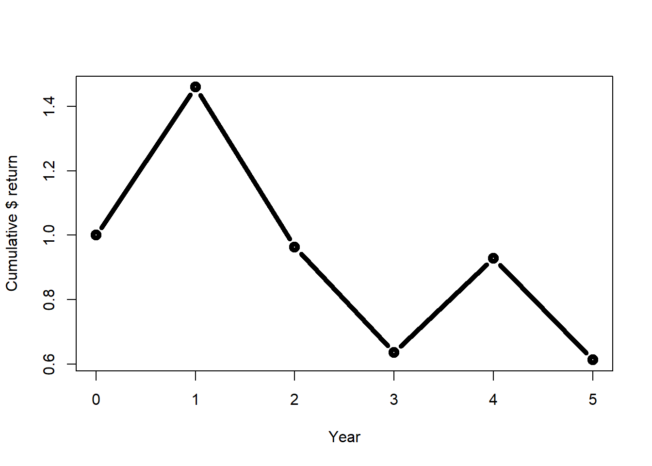
The evolution of $1 dollar invested in this 5 year period would look like this:
Figure 2.27: 5-year simulation of cumulative returns for asset A.
Even simpler and quicker, a \(\$1\) dollar invested at \(t=0\) would lead to \(\$0.6128265\) at \(t=5\).
Code
prod(a)
[1] 0.6128265
Let’s use a function now.
Code
binomial_tree <-function(u, d, n) {prod(sample(c(1+u, 1-d), n, replace =TRUE))}
See if it works. Calculate the asset A cumulative return of a 5-year and 30-year investment.
Code
set.seed(2, sample.kind ="Rounding")binomial_tree(u =0.46, d =0.34, n =5)
[1] 0.6128265
Code
set.seed(2, sample.kind ="Rounding")binomial_tree(u =0.46, d =0.34, n =30)
[1] 2.805884
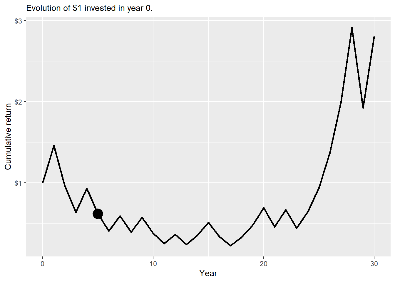
It works, a \(\$1\) dollar invested at \(t=0\) would lead to \(\$0.6128265\) in 5 years as we show before. And now we know that a \(\$1\) dollar invested at \(t=0\) would lead \(\$2.805884\) in 30 years. Let’s view the 30 year case:
Code
u =0.46d =0.34n =30set.seed(2, sample.kind ="Rounding")a.30<-c(1, cumprod(sample(c(1+u, 1-d), n, replace =TRUE)))a.30<-as.data.frame(cbind(year =c(0:30), ret = a.30))ggplot(a.30, aes(x = year, y = ret)) +geom_line(size =1) +geom_point(aes(x =5, y =0.6128265), size =6) +labs(y ="Cumulative return", x ="Year",subtitle ="Evolution of $1 invested in year 0.") +scale_y_continuous(labels = scales::dollar)
Figure 2.28: 30-year cumulative return asset A.
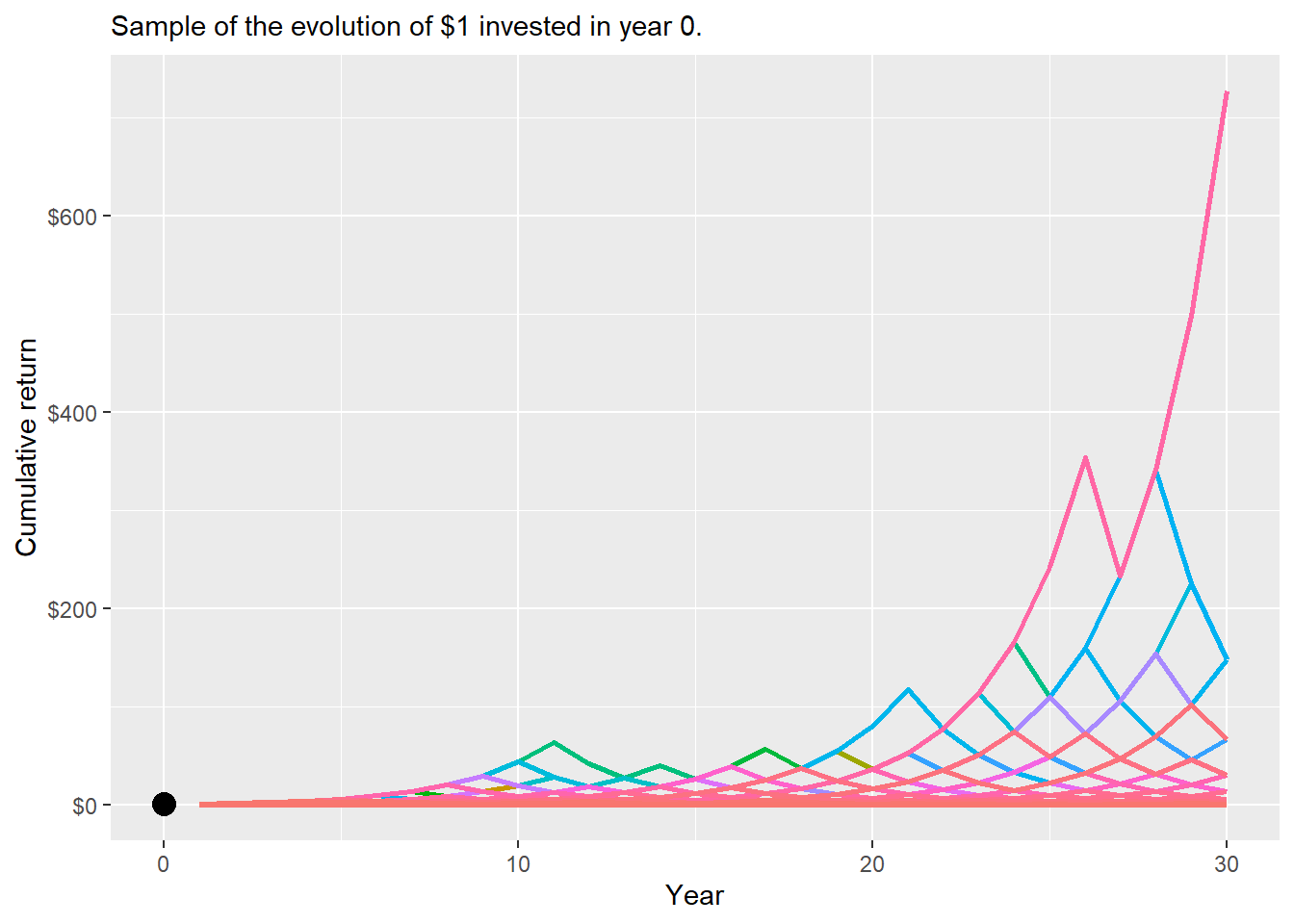
These results represent one single path. To understand a typical terminal value, we need to simulate many paths and summarize the terminal distribution. Let’s simulate 10,000 paths and estimate the median value of our \(\$1\) dollar investment in 30 years.
Code
u =0.46d =0.34n =30set.seed(2, sample.kind ="Rounding")a.30x10k <-replicate(10000, cumprod(sample(c(1+u, 1-d), n, replace =TRUE))) |>as.data.frame() |>mutate(year =c(1:30)) |>gather(V1:V10000, key = name, value = c.ret)set.seed(2, sample.kind ="Rounding")plot_paths <- a.30x10k |>distinct(name) |>slice_sample(n =1000)
See a representative sample of the simulated paths.
Code
a.30x10k |>semi_join(plot_paths, by ="name") |>ggplot(aes(x = year, y = c.ret, color = name)) +geom_line(size =1) +geom_point(aes(x =0, y =1), col ="black", size =4) +theme(legend.position ="none", legend.title =element_blank()) +labs(y ="Cumulative return", x ="Year",subtitle ="Sample of the evolution of $1 invested in year 0.") +scale_y_continuous(labels = scales::dollar)
Figure 2.29: 30-year cumulative return asset A, sample of simulated paths.
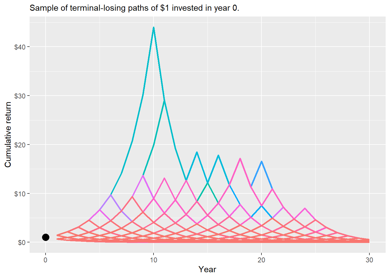
Most of these paths are concentrated in low cumulative returns by the end of the 30 years. The following code counts paths with a terminal cumulative return lower than $1:
a.30x10k |>semi_join(losing_paths_plot, by ="name") |>ggplot(aes(x = year, y = c.ret, color = name)) +geom_line(size =1) +geom_point(aes(x =0, y =1), col ="black", size =4) +theme(legend.position ="none", legend.title =element_blank()) +labs(y ="Cumulative return", x ="Year",subtitle ="Sample of terminal-losing paths of $1 invested in year 0.") +scale_y_continuous(labels = scales::dollar)
Figure 2.30: 30-year cumulative return asset A, sample of terminal-losing paths.
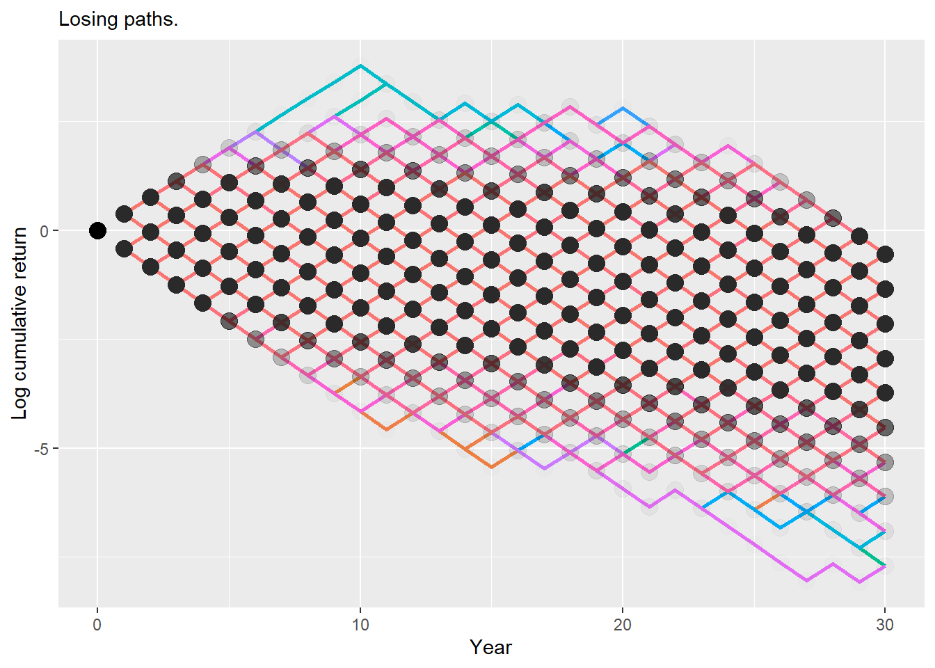
The figure above looks still unclear as the concentration around $0 is still high. It is better to show the results in logarithm form.
Code
a.30x10k |>semi_join(losing_paths_plot, by ="name") |>ggplot(aes(x = year, y =log(c.ret), color = name)) +geom_line(size =1) +geom_point(col ="black", alpha =0.01, size =4) +geom_point(aes(x =0, y =log(1)), col ="black", size =4) +theme(legend.position ="none", legend.title =element_blank()) +labs(y ="Log cumulative return", x ="Year",subtitle ="Losing paths.")
Figure 2.31: 30-year log cumulative return asset A, sample of terminal-losing paths.
The figure now resembles a binomial tree. The black circles are more transparent for less concentrated values and less transparent for more concentrated values.
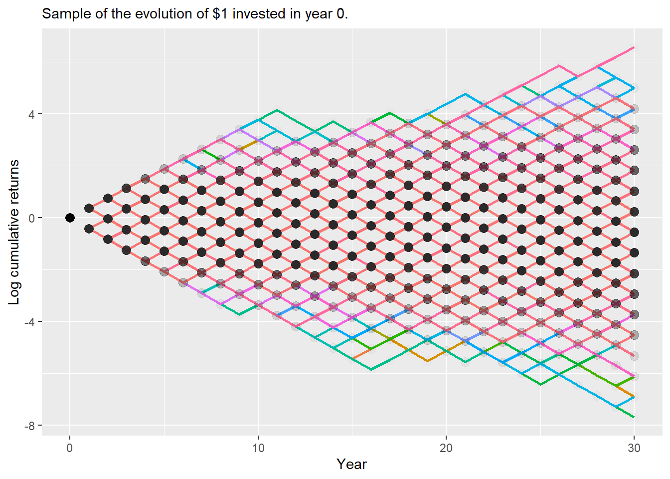
Let’s do a similar plot for the same representative sample.
Code
a.30x10k |>semi_join(plot_paths, by ="name") |>ggplot(aes(x = year, y =log(c.ret), color = name)) +geom_line(size =1) +geom_point(aes(x =0, y =log(1)), size =3, col ="black") +geom_point(col ="black", alpha =0.01, size =3) +theme(legend.position ="none", legend.title =element_blank()) +labs(y ="Log cumulative returns", x ="Year",subtitle ="Sample of the evolution of $1 invested in year 0.")
Figure 2.32: 30-year Log cumulative return asset A, sample of simulated paths.
Here it is easier to see that the paths actually follow a binomial structure. Now, let’s see the summary statistics for the 10,000 possible investment value at year 30.
Code
set.seed(2, sample.kind ="Rounding")summary(replicate(10000, binomial_tree(u =0.46, d =0.34, 30)))
     Min.   1st Qu.    Median      Mean   3rd Qu.      Max.
   0.0001    0.1172    0.5734    5.8157    2.8059 3559.1803
The median terminal value of our 30-year investment of \(\$1\) in this asset A with 6% expected return and 40% volatility is below the initial investment. Even if we drop the set.seed(), the median remains close to this value.
Code
median(replicate(10000, binomial_tree(u =0.46, d =0.34, 30)))
[1] 0.5733923
The mean and the median answer different questions. The mean terminal value is close to \((\$1+0.06)^{30}=\$5.743491\), while the median represents the typical terminal outcome of the simulated paths.
Code
(1+0.06)^30
[1] 5.743491
Under a median terminal-wealth criterion, asset A is a losing investment: \(\$1\) would typically lead to about \(\$0.5733923\) in 30 years.
Now, let’s consider an asset B. Asset B has a known excess return of \(-0.1\%\). In the context of a binomial tree:
\(0.5(1+u)+0.5(1-d)=0.999\).
Asset B has no volatility, imagine is a Treasury Bill or a similar risk-free asset. Solving for \((1+u)\) and \((1-d)\) leads to \((1+u)=0.999\) and \((1-d)=0.999\). Asset B is a losing investment as well.
In a period of 5 years, we would have a random path of ups and downs in the context of a binomial path. Although in this case the result is the same as we have no risk.
Code
b <-sample(c(1+(-0.001), 1-(0.001)), 5, replace =TRUE)b
[1] 0.999 0.999 0.999 0.999 0.999
The evolution of $1 dollar invested in this 5-year period would look like this:
Code
cumprod(b)
[1] 0.999000 0.998001 0.997003 0.996006 0.995010
Or simply:
Code
prod(b)
[1] 0.99501
As stated earlier, this asset B is a losing investment. Let’s verify this for 5 and 30 years as we did before for the case of asset A:
Code
binomial_tree <-function(u, d, n) {prod(sample(c(1+u, 1-d), n, replace =TRUE))}set.seed(2, sample.kind ="Rounding")binomial_tree(u = (-0.001), d = (0.001), 5)
[1] 0.99501
Code
binomial_tree(u = (-0.001), d = (0.001), 30)
[1] 0.970431
It works, a \(\$1\) dollar invested at \(t=0\) would lead to \(\$0.99501\) in 5 years. And now we know that a \(\$1\) dollar invested at \(t=0\) would lead to \(\$0.970431\) in 30 years. These results represent one single path, but we do not need more as there is no risk. Let’s confirm:
Code
set.seed(2, sample.kind ="Rounding")median(replicate(10000, binomial_tree(u =-0.001, d =0.001, 30)))
[1] 0.970431
The result is the same. Asset B is a losing investment as well. But, what if we combine both assets A and B in an equally weighted portfolio C?
Code
set.seed(2, sample.kind ="Rounding")median(replicate(1, binomial_tree(u = (0.46-0.001)/2, d = (0.34+0.001)/2, 30)))
[1] 2.951197
This is how we combine two losing investments into a winner.
The new asset C or portfolio C has an expected arithmetic return of \(0.06/2 - 0.001/2=0.0295\), or \(2.95\%\).
The volatility of C is \(\sqrt{0.5^2(0.4)^2+0.5^2(0)^2-0}=0.2\) or \(20\%\).
Therefore, portfolio C has a lower expected arithmetic return and lower risk than asset A. Because B is deterministic, its variance is zero and its covariance contribution is zero; the portfolio variance comes from half exposure to asset A. Under the median terminal-wealth criterion, we can combine two losing investments into a winner.
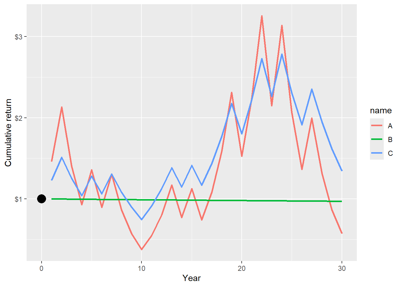
Let’s visualize how these assets behave. I have to set the seed to have nice results. As shown before, this works well when simulating many paths and computing the median terminal cumulative return of each asset.
Below, it is clear that portfolio C wins less when asset A wins. Similarly, portfolio C loses less when asset A loses. This is because portfolio C is less risky than asset A.
Code
abc <-as.data.frame(cbind(year =c(1:30), A =cumprod(a30), B =cumprod(b30), C =cumprod(c30)))head(abc)
  year         A        B        C
1    1 1.4600000 0.999000 1.229500
2    2 2.1316000 0.998001 1.511670
3    3 1.4068560 0.997003 1.253930
4    4 0.9285250 0.996006 1.040135
5    5 1.3556464 0.995010 1.278846
6    6 0.8947267 0.994015 1.060803
This is the cumulative return evolution for each asset and portfolio C in one single path.
Code
abc |>gather(A:C, key = name, value = c.ret) |>ggplot(aes(x = year, y = c.ret, color = name)) +geom_line(size =1) +geom_point(aes(x =0, y =1), size =5, col ="black") +labs(y ="Cumulative return", x ="Year") +scale_y_continuous(labels = scales::dollar)
Figure 2.33: 30-year cumulative returns asset A, B and portfolio C, one single path.
Now we plot the 10,000 possible values of the 30 year cumulative returns.
Code
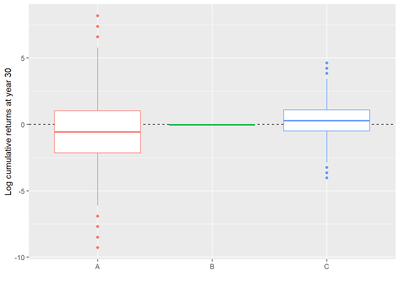
set.seed(2, sample.kind ="Rounding")bx <- (replicate(10000, binomial_tree(u =-0.001, d =0.001, 30)))set.seed(2, sample.kind ="Rounding")cx <- (replicate(10000, binomial_tree(u = (0.46-0.001)/2, d = (0.34+0.001)/2, 30)))set.seed(2, sample.kind ="Rounding")ax <-(replicate(10000, binomial_tree(u =0.46, d =0.34, 30)))abcx <-as.data.frame(cbind(simulation =c(1:10000), A = ax, B = bx, C = cx))abcx |>gather(A:C, key = name, value = c.ret) |>ggplot(aes(x = name, y =log(c.ret), color = name)) +geom_hline(yintercept =0, lty =2) +geom_boxplot() +theme(legend.position ="none") +labs(y ="Log cumulative returns at year 30", x ="")
Figure 2.34: 30-year log cumulative returns asset A, B and portfolio C, only the final cumulative return.
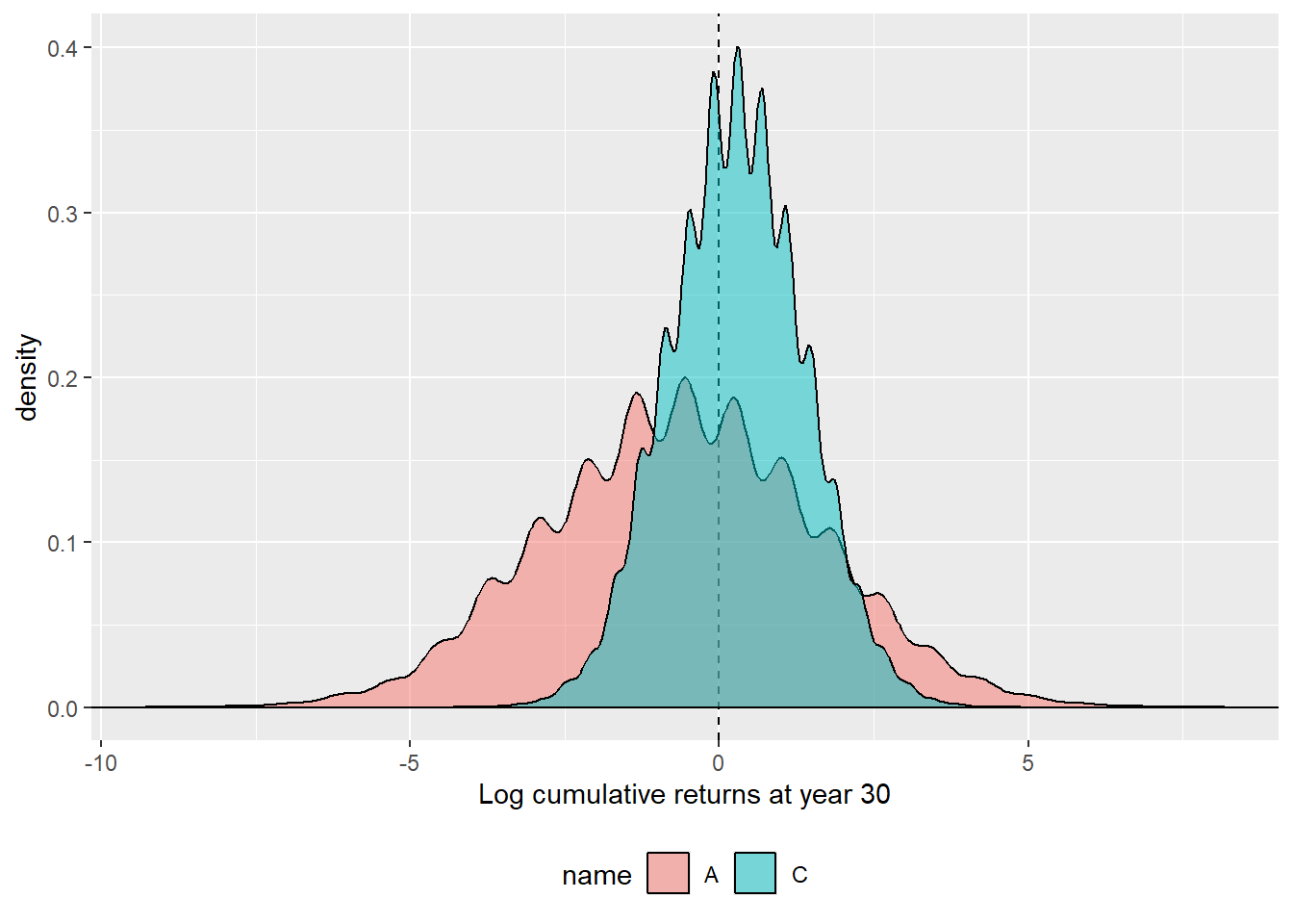
An alternative to the boxplot is a density plot.
Code
abcx |>gather(A:C, key = name, value = c.ret) |>filter(name %in%c("A", "C")) |>ggplot(aes(x =log(c.ret), fill = name)) +geom_vline(xintercept =0, lty =2) +geom_density(alpha =0.5) +theme(legend.position ="bottom") +labs(x ="Log cumulative returns at year 30") +geom_hline(yintercept =0)
Figure 2.35: 30-year log cumulative returns asset A and portfolio C, only the final cumulative return, a density view.
Stock price paths are useful to value option stocks. Let’s review some stochastic processes in the next section.
Hull, John C. 2015. Options, Futures, and Other Derivatives. 9th ed. Prentice Hall.