3 Wiener processes

Here we review stochastic process that are useful in finance, especially in the Black-Scholes context. This section is based on Hull (2015), chapter 14.

3.1 The basic process

A simple Wiener process.

Code

# A typical Wiener process.
TT <- 5
N <- 10000
dt <- TT / N
Time <- seq(from = dt, to = TT, by = dt)
set.seed(560746) # for reproducibility purposes.
delta_z <- rnorm(N, 0, 1) * dt^0.5 
z <- 25 + cumsum(delta_z) # The initial price is 25.

Graphically:

Code

plot(Time, z, type = "l",
     ylab = "z in the texbook, it could be a stock price",
     xlab = "Time")
lines(Time, seq(25, (25 + sum(delta_z)), length.out = N), lty = 2,
      col = "purple")
points(Time[1], 25, col = "blue", cex = 2, pch = 16)
points(Time[N], z[N], col = "red", cex = 2, pch = 16)
legend("topleft", legend = c(round(z[N], 2)), bg = "white", 
       text.col = "red")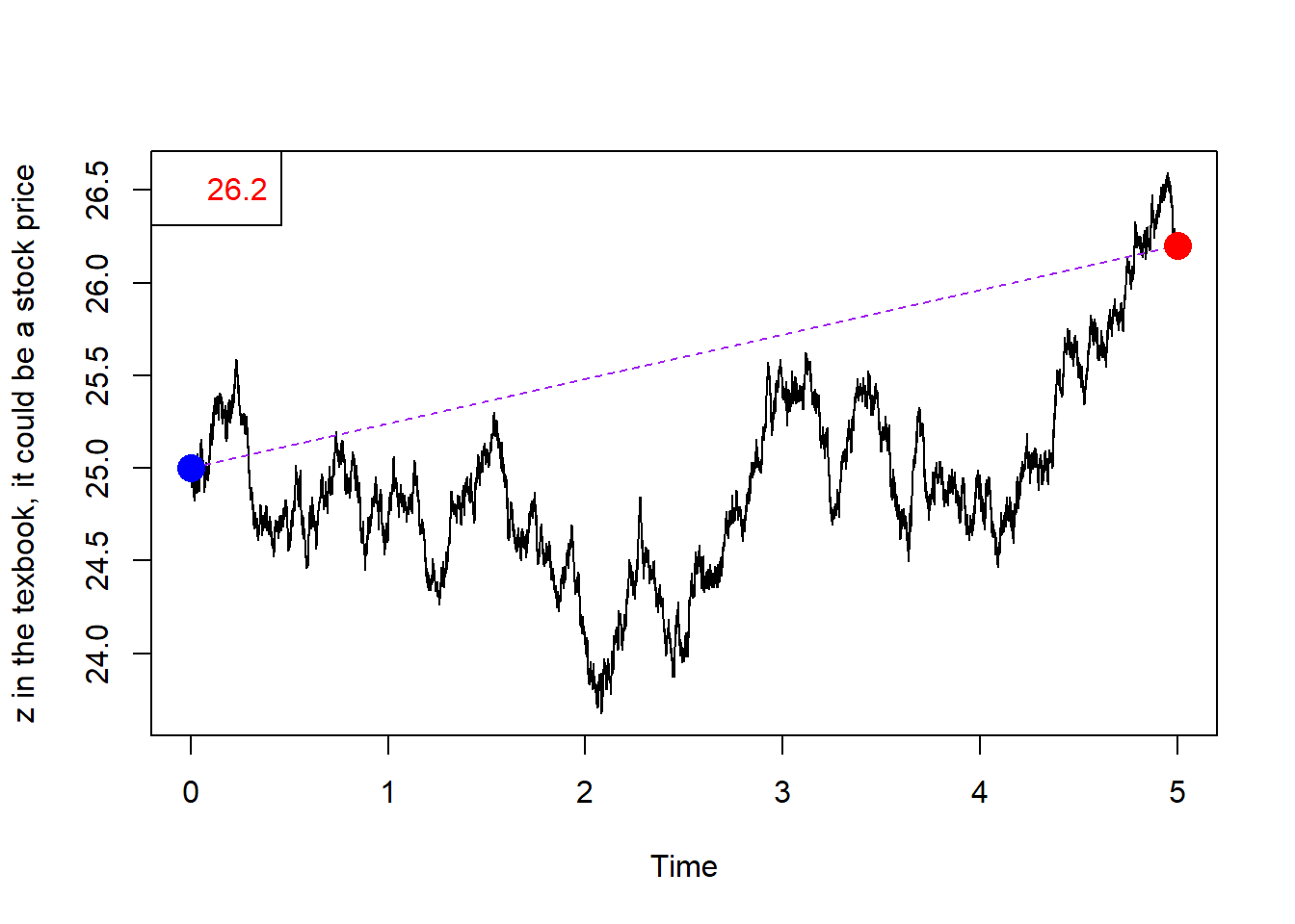

Figure 3.1: Wiener process 10,000 steps from blue $z(0)=25$ to $z(T)=26.2$ in red.

This is a 1,000 step version of four Wiener processes:

Code

embed_url("https://youtu.be/X-VRWeqG_I8")

This is supposed to mimic (at some extent) the evolution of a stock price.

Now, we propose to produce 100 processes.

Code

# 100 Wiener processes.
set.seed(365633)
mat.delta_z <- matrix(rnorm(100 * N, mean = 0, sd = 1) * sqrt(dt), 100, N) 
mat.z1 <- 25 + t(apply(mat.delta_z, 1, cumsum)) 
mat.z <- t(cbind(matrix(25, 100), mat.z1))
Time2 <- c(0, Time)
pred <- mean(mat.z[(N + 1), ])
# 95% range.
rangetop <- pred + qnorm(0.975) * var(mat.z[(N + 1), ])^0.5
rangedown <- pred - qnorm(0.975) * var(mat.z[(N + 1), ])^0.5

Graphically.

Code

matplot(Time2, mat.z, type = "l", lty = 1, col = rgb(0, 0, 1, 0.3),
     ylab = "z in the textbook, it could be a stock price",
     xlab = "Time")
abline(h = pred, lty = 2, col = "red")
abline(v = 0, lty = 2)
lines(Time2, seq(25, pred, length.out = N + 1), lty = 2)
points(Time2[N + 1], pred, col = "red", cex = 2, pch = 16)
points(0, 25, col = "black", cex = 2, pch = 16)
legend("topleft", legend = c(round(pred, 2)), bg = "white", 
       text.col = "red")
abline(h = rangetop, lty = 2)
abline(h = rangedown, lty = 2)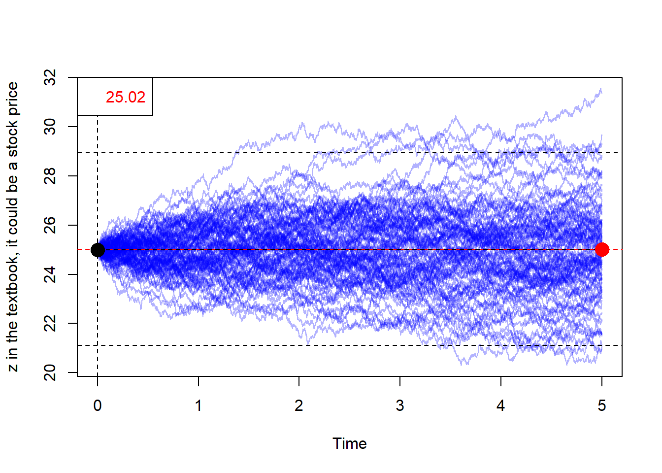

Figure 3.2: 100 Wiener process 10,000 steps, initial price at 25, red is the mean at $T$.

Let’s check how many simulated terminal values fall outside this 95% prediction range.

Code

sum(mat.z[(N + 1), ] > rangetop)

[1] 3

Code

sum(mat.z[(N + 1), ] < rangedown)

[1] 2

This means that 5 paths are outside this simulated 95% prediction range.

Code

summary(mat.z[(N + 1), ])

   Min. 1st Qu.  Median    Mean 3rd Qu.    Max. 
  20.97   23.79   24.96   25.02   26.06   31.38

A potential problem is that $z$ values can be negative. This is problematic when we are interested to model stock prices.

Let’s explore deeper the stochastic process below.

Code

set.seed(1)
delta_z <- rnorm(N, 0, 1) * dt^0.5 
z <- 25 + cumsum(delta_z)
### A stochastic process
par(mfrow = c(2, 2), mai = c(0.4, 0.4, 0.4, 0.4))
par(pty = "s")
plot(Time, z, type = "l", xlim = c(0, TT), ylim = c(22.5, 26),
     main = "Full 5-year period", ylab = "z", xlab = "Time")
plot(Time, delta_z, type = "h", xlim = c(0, TT),
     main = "Full 5-year period", 
     ylab = expression(paste(Delta,z)), xlab = "Time")
abline(h = 0, lty = 2, col = "orange", lwd = 2)
plot(Time, z, type = "l", xlim = c(0, 1/12), ylim = c(24.9, 25.35),
     main = "Zoom: first month only", xlab = "Time")
plot(Time, delta_z, type = "h", xlim = c(0, 1/12), 
     col = ifelse(delta_z < 0, "red", "blue"), ylim = c(-0.055, 0.055),
     main = "Zoom: first month only", 
     ylab = expression(paste(Delta,z)), xlab = "Time")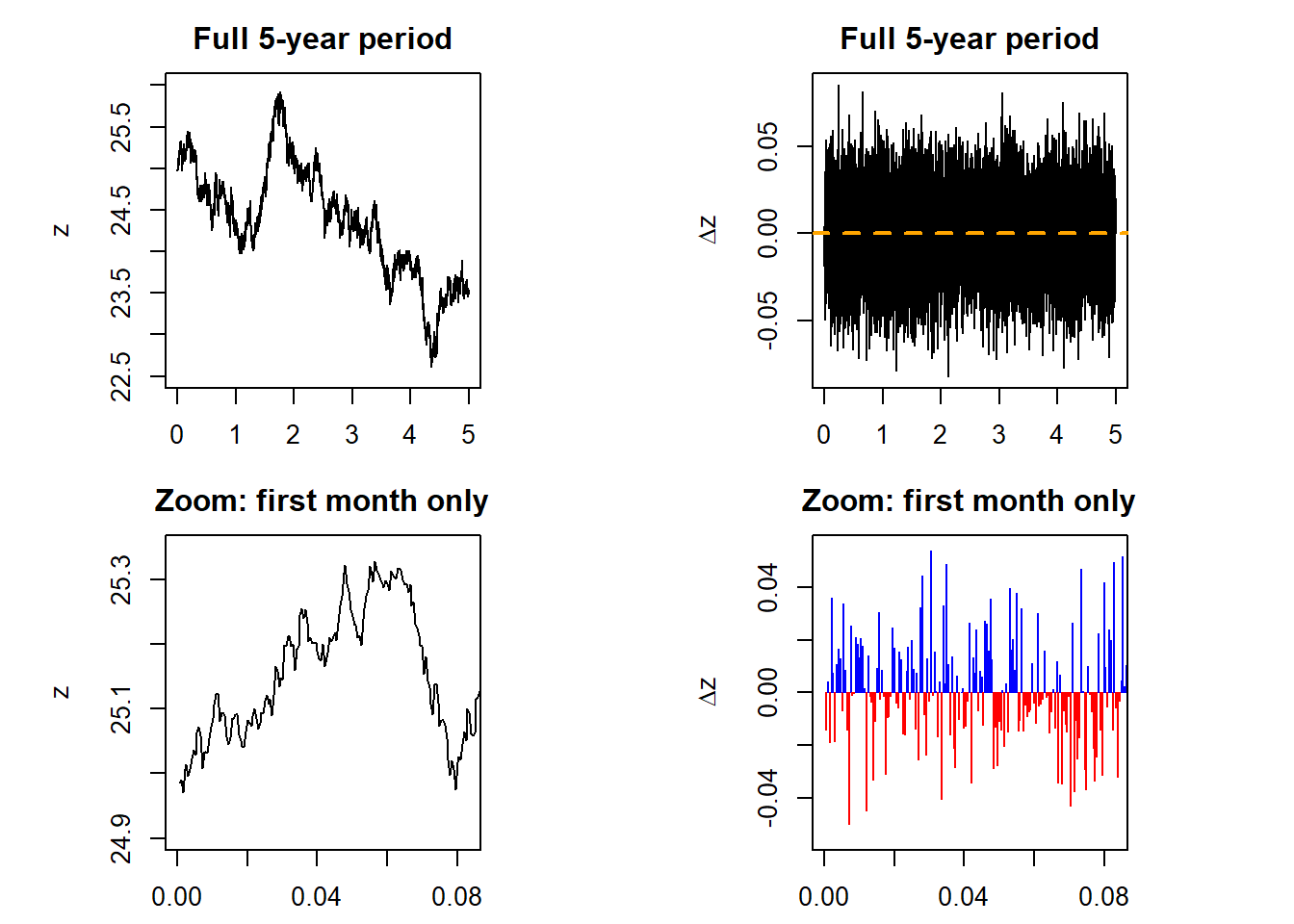

Figure 3.3: A stochastic process with zoom.

These processes are driven by a random component. The lower panel is revealing because we can see how the random component goes from positive to negative without any pattern, it is entirely random. Now, let’s explore the role of $\Delta t$.

Code

par(mfrow = c(2, 2), mai = c(0.4, 0.4, 0.4, 0.4))
par(pty = "s")
plot(Time[(seq(from = 1, to = N, length.out = 10))],
     z[(seq(from = 1, to = N, length.out = 10))], type = "l",
     ylim = c(22.5, 26), main = expression(paste("Large ",Delta,t)),
     ylab = "z")
abline(v = 0, lty = 2)
abline(v = 5, lty = 2)
plot(Time[(seq(from = 1, to = N, length.out = 100))],
     z[(seq(from = 1, to = N, length.out = 100))], type = "l", 
     ylim = c(22.5, 26), ylab = "z", 
     main = expression(paste("Small ",Delta,t)))
abline(v = 0, lty = 2)
abline(v = 5 , lty = 2)
plot(Time[(seq(from = 1, to = N, length.out = 1000))],
     z[(seq(from = 1, to = N, length.out = 1000))], type = "l", 
     ylim = c(22.5, 26), ylab = "z", 
     main = expression(paste("Even smaller ",Delta,t)))
abline(v = 0, lty = 2)
abline(v = 5 , lty = 2)
plot(Time, z, type = "l", ylim = c(22.5, 26), # length 10,000
     main = expression(paste("True process ",Delta,t, " ",
                             "tends ","to ","zero")))
abline(v = 0, lty = 2)
abline(v = 5, lty = 2)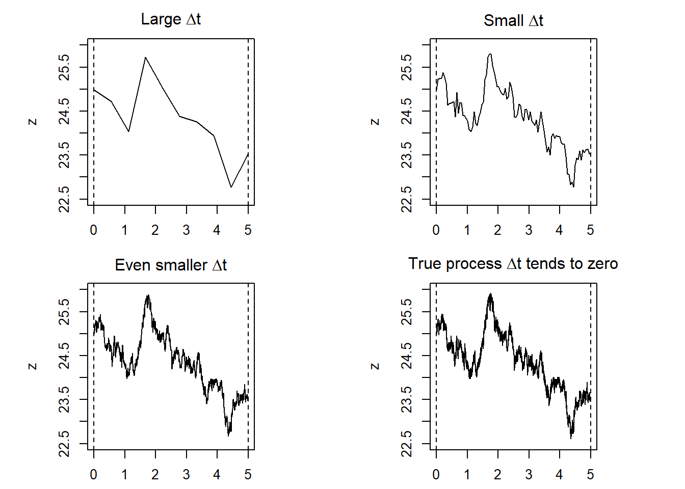

Figure 3.4: Wiener process, the role of $\Delta t$.

The $\Delta t$ value determines how frequent are the changes in $z$.

A few properties of stochastic processes.

Code

mean(delta_z) # should be zero

[1] -0.0001461726

Code

var(delta_z)^0.5 # should be dt^.5

[1] 0.02263698

Code

dt^0.5

[1] 0.02236068

Code

var(delta_z) # should be dt

[1] 0.0005124328

Code

dt

[1] 5e-04

3.2 The generalized Wiener process

Now let’s analyze the case of the generalized Wiener process.

$\Delta x = a \Delta t + b \epsilon \sqrt{\Delta t}$. Assume $a=0.3$ and $b=1.5$:

Code

# Figure 14.2
TT <- 50
N <- 200
dt <- TT / N
Time <- seq(from = 0, to = TT, by = dt)
set.seed(123)
delta_z <- 1.5 * rnorm(N, 0, 1) * dt^0.5
delta_x <- (0.3 * dt) + delta_z
x <- c(0, cumsum(delta_x))
z <- c(0, cumsum(delta_z))

Graphically:

Code

plot(Time, x, type = "l", lwd = 4, ylim = c(-7, 22))
lines(Time, z, col = "red", lwd = 4)
lines(Time, 0.3 * Time, col = "blue", lwd = 4)
abline(0, 0)
abline(v = 0)
legend("topleft", legend = c("Generalized Wiener process", 
                             "Drift", "Stochastic component"),
       col = c("black", "blue", "red"), lwd = 3, 
       bg = "white", cex = 0.8)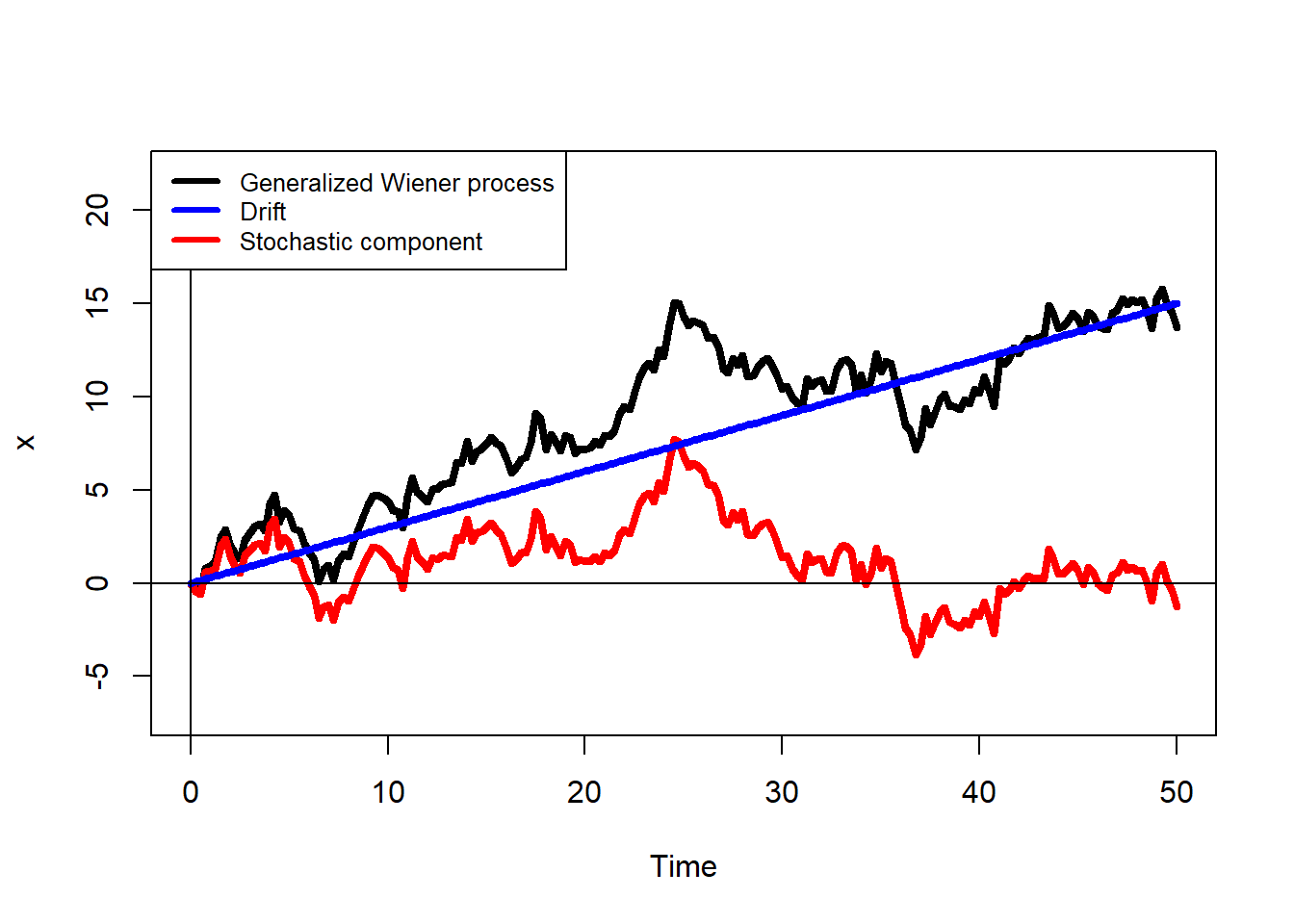

Here, the generalized Wiener process $\Delta x$ is decomposed into the drift $a \Delta t$ and the stochastic component $b \epsilon \sqrt{\Delta t}$. A zoom of the same plot.

Code

# Figure 14.2 Zoom
plot(Time, x, type = "b", ylim = c(-0.6, 1), xlim = c(0, 1), lwd = 4)
lines(Time, z, col = "red", lwd = 4, type = "b")
lines(Time, 0.3 * Time, col = "blue", lwd = 4, type = "b")
abline(0, 0)
abline(v = 0)
abline(v = dt, lty = 2)
abline(v = dt * 2, lty = 2)
abline(v = dt * 3, lty = 2)
abline(v = dt * 4, lty = 2)
#points(dt, 0, pch = 1, col = "blue", lwd = 2)
#points(dt * 2, 0, pch = 1, col = "blue", lwd = 2)
#points(dt * 3, 0, pch = 1, col = "blue", lwd = 2)
#points(dt * 4, 0, pch = 1, col = "blue", lwd = 2)
legend("topleft", legend = c("Generalized Wiener process", 
                           "Drift", "Stochastic component"),
       col = c("black", "blue", "red"), lty = 1, 
       bg = "white", lwd = 2)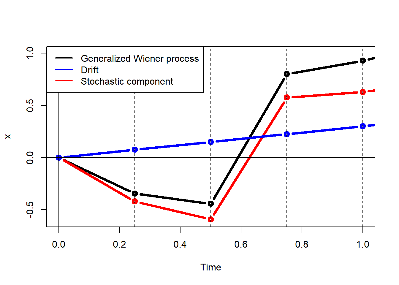

Figure 3.6: Generalized Wiener process, zoom view.

This is a nice visual representation of: generalized = drift + Wiener.

See how the process changes when we consider a lower value of $a$.

Code

set.seed(123)
delta_xlow <- (0.15 * dt) + delta_z
xlow <- c(0, cumsum(delta_xlow))
# Now plot.
plot(Time, xlow, type = "l", ylim = c(-7, 22), lwd = 4, ylab = "x")
lines(Time, x, lwd = 2, col = "grey")
lines(Time, z, lwd = 4, col = "red")
lines(Time, 0.15 * Time, lwd = 4, col = "blue")
lines(Time, 0.3 * Time, lty = 2, lwd = 2, col = "grey")
abline(0, 0)
abline(v = 0)
legend("topleft", legend = c("Original generalized Wiener process", 
    "Original drift", "New generalized Wiener process", "New drift",
    "Stochastic component"), lty = c(1, 2, 1, 1, 1), 
    bg = "white", lwd = 2,
    col = c("grey", "grey", "black", "blue", "red"), cex = 0.85)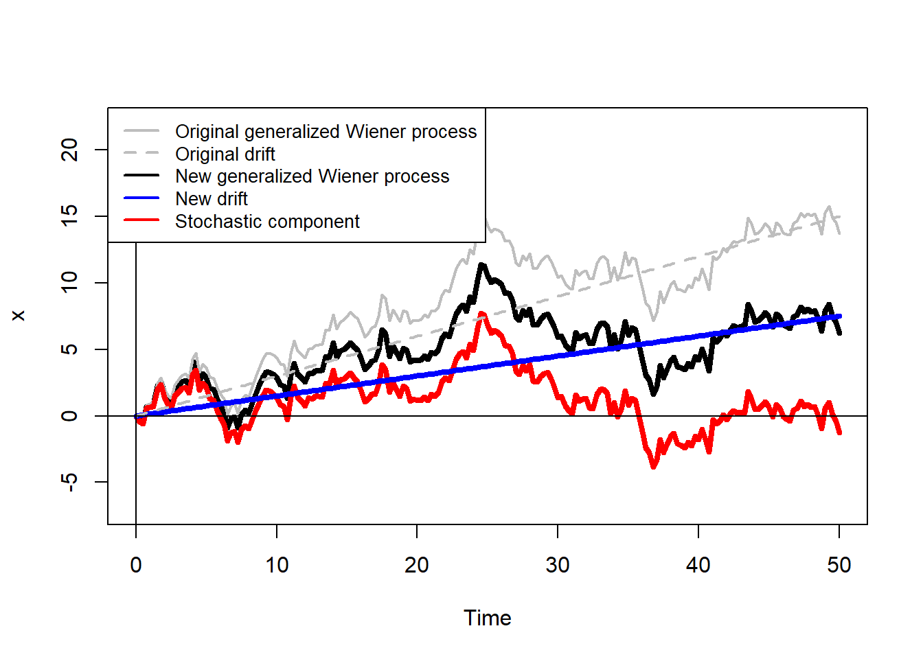

Figure 3.7: Generalized Wiener process, lower a.

And a higher value of $b$.

Code

set.seed(123)
delta_zhigh <- 3 * rnorm(N, 0, 1) * dt^0.5
delta_xhigh <- (0.3 * dt) + delta_zhigh
xhigh <- c(0, cumsum(delta_xhigh))
zhigh <- c(0, cumsum(delta_zhigh))
plot(Time, xhigh, type = "l", ylim = c(-7, 22), lwd = 4, ylab = "x")
lines(Time, x, lwd = 2, col = "grey")
lines(Time, zhigh, lwd = 4, col = "red")
lines(Time, z, lwd = 2, col = "grey")
lines(Time, 0.3 * Time, lwd = 4, col = "blue")
abline(0, 0)
abline(v = 0)
legend("topleft", legend = c("New generalized Wiener process", 
      "Original generalized Wiener process", "Drift" ,
      "New stochastic component", "Original stochastic component"), 
      lty = 1, bg = "white", lwd = 2,
      col = c("black", "grey", "blue", "red", "grey"), cex = 0.75)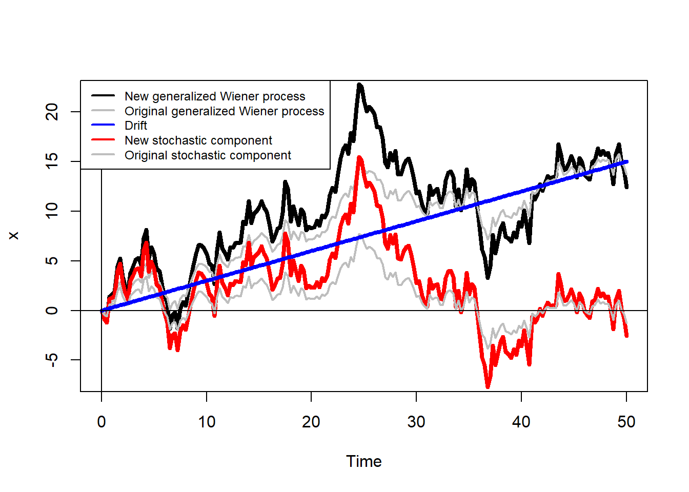

Figure 3.8: Generalized Wiener process, higher b.

Note the changes are now more pronounced.

This is a replication of Hull (2015), table 14.1. Simulation of stock price when $\mu= 0.15$ and $\sigma = 0.30$ during 1-week periods.

Code

# Table 14.1
set.seed(19256)
delta_S <- rep(0, 10)
S <- rep(100, 10)
epsilon <- rep(0, 10)
for(i in 1:10){
  epsilon[i] <- rnorm(1, 0, 1)
  delta_S[i] <- 0.15 * (1 / 52) * S[i] + 0.3 * ((1 / 52)^0.5) * 
    epsilon[i] * S[i]
  S[i+1] <- S[i] + delta_S[i]
}
epsilon <- c(epsilon, NA)
delta_S <- c(delta_S, NA)
results <- data.frame(S, epsilon, delta_S)
results

          S    epsilon    delta_S
1  100.0000  0.8268625  3.7284174
2  103.7284  0.4957988  2.4387684
3  106.1672 -0.9313823 -3.8074983
4  102.3597 -0.1495925 -0.3417592
5  102.0179  0.7310239  3.3968957
6  105.4148 -0.6111472 -2.3761181
7  103.0387  1.2490868  5.6516490
8  108.6904 -0.6243389 -2.5096009
9  106.1808  0.6995349  3.3964067
10 109.5772  0.3612549  1.9629353
11 111.5401         NA         NA

It is interesting to note that in Hull (2015) the final simulated price is $111.54 and here it is $111.5401. Is this a pure coincidence?

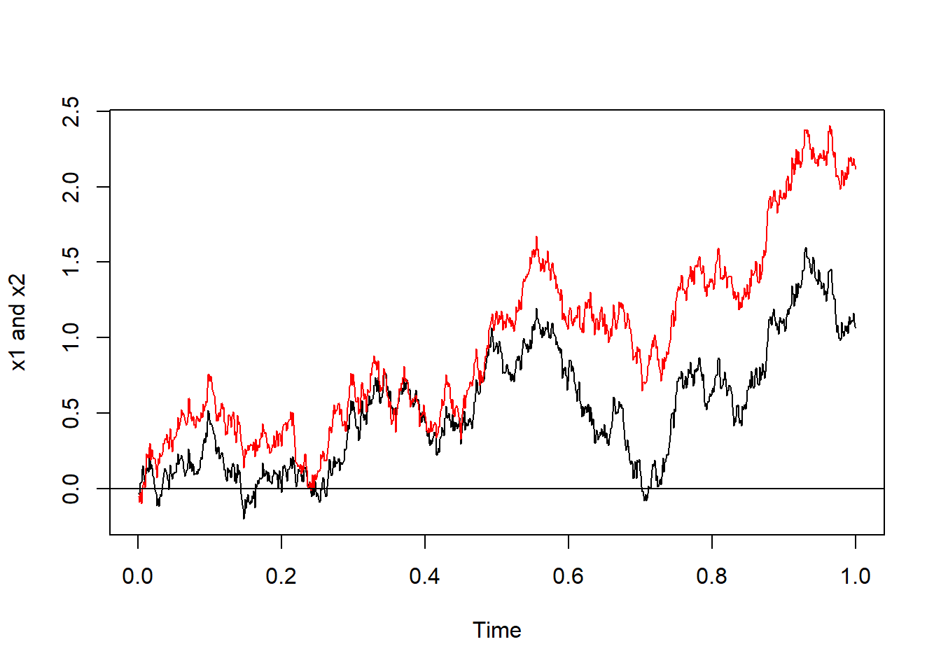
A correlated process.

$\Delta x_1 = a_1 \Delta t + b_1 \epsilon_1 \sqrt{\Delta t}$,

$\Delta x_2 = a_2 \Delta t + b_2 \epsilon_2 \sqrt{\Delta t}$.

Where: $\epsilon_1 = u$, and $\epsilon_2=\rho u + \sqrt{1-\rho^{2}}v$.

Code

# Section 14.5
rho <- 0.8
TT <- 1
steps <- 1000
dt <- TT / steps
Time <- seq(from = dt, to = TT, by = dt)
set.seed(123)
e1 <- rnorm(steps, 0, 1)
e2 <- rho * e1 + ((1 - rho^2)^0.5) * rnorm(steps, 0, 1)
delta_z1 <- 1.5 * e1 * dt^0.5
delta_z2 <- 1.5 * e2 * dt^0.5
delta_x1 <- (0.3 * dt) + delta_z1
delta_x2 <- (0.3 * dt) + delta_z2
x1 <- cumsum(delta_x1)
x2 <- cumsum(delta_x2)
x <- c(x1, x2)

Assume $a=0.3$, $b=1.5$ and $\rho=0.8$. Visually:

Code

plot(Time, x1, type = "l", ylim = c(min(x), max(x)), ylab = "x1 and x2")
lines(Time, x2, col = "red")
abline(0, 0)

Figure 3.9: Correlated processes x1 and x2.

The model of stock price behavior implies that a stock’s price at time $T$, given its price today, is lognormally distributed. The following is similar to example 15.1 in Hull (2015). In particular, consider a stock with an initial price of $40, an expected return of 16% per annum, and a volatility of 20% per annum.

$\frac{\Delta S}{S} = a \Delta t + b \epsilon \sqrt{\Delta t}$,

$\frac{\Delta S}{S} = 0.16 \Delta t + 0.2 \epsilon \sqrt{\Delta t}$,

Assume $\Delta t = \frac{1}{365}$: $\frac{\Delta S}{S} = 0.16 \frac{1}{365} + 0.2 \epsilon \sqrt{\frac{1}{365}}$,

Calculate the constants:

Code

0.16/365

[1] 0.0004383562

Code

0.2*(1/365)^0.5

[1] 0.01046848

Finally: $\Delta S = 0.0004383562 S + 0.01046848 S \epsilon$. The 100 simulated 6-months paths of the stock price $S$ are:

Code

set.seed(10101010)
for(j in 1:100) {
  delta_S <- NULL 
  S <- rep(40, 180) # Now it is 40 for all days, the loop fill this out.
  epsilon <- NULL 
  for(i in 1:180) {
    epsilon[i] <- rnorm(1, 0, 1)
    delta_S[i] <- 0.16 * (1 / 365) * S[i] + 0.2 * ((1 / 365)^0.5) *
      epsilon[i] * S[i]
    S[i+1] <- S[i] + delta_S[i]
    }
  if (j==1) {
    plot(S, type = "l", ylim = c(30, 60), 
         ylab = expression(paste(S[t])), xlab = "t (days)")
    points(0, 40, pch = 19, col = "blue", cex = 3)
    abline(h = 10, col = "red", lwd = 3)
    }
  lines(S)
  }
abline(h = 32.55, lwd = 2, col = "red")
abline(h = 56.56, lwd = 2, col = "red")
abline(v = 181, lwd = 2, col = "red")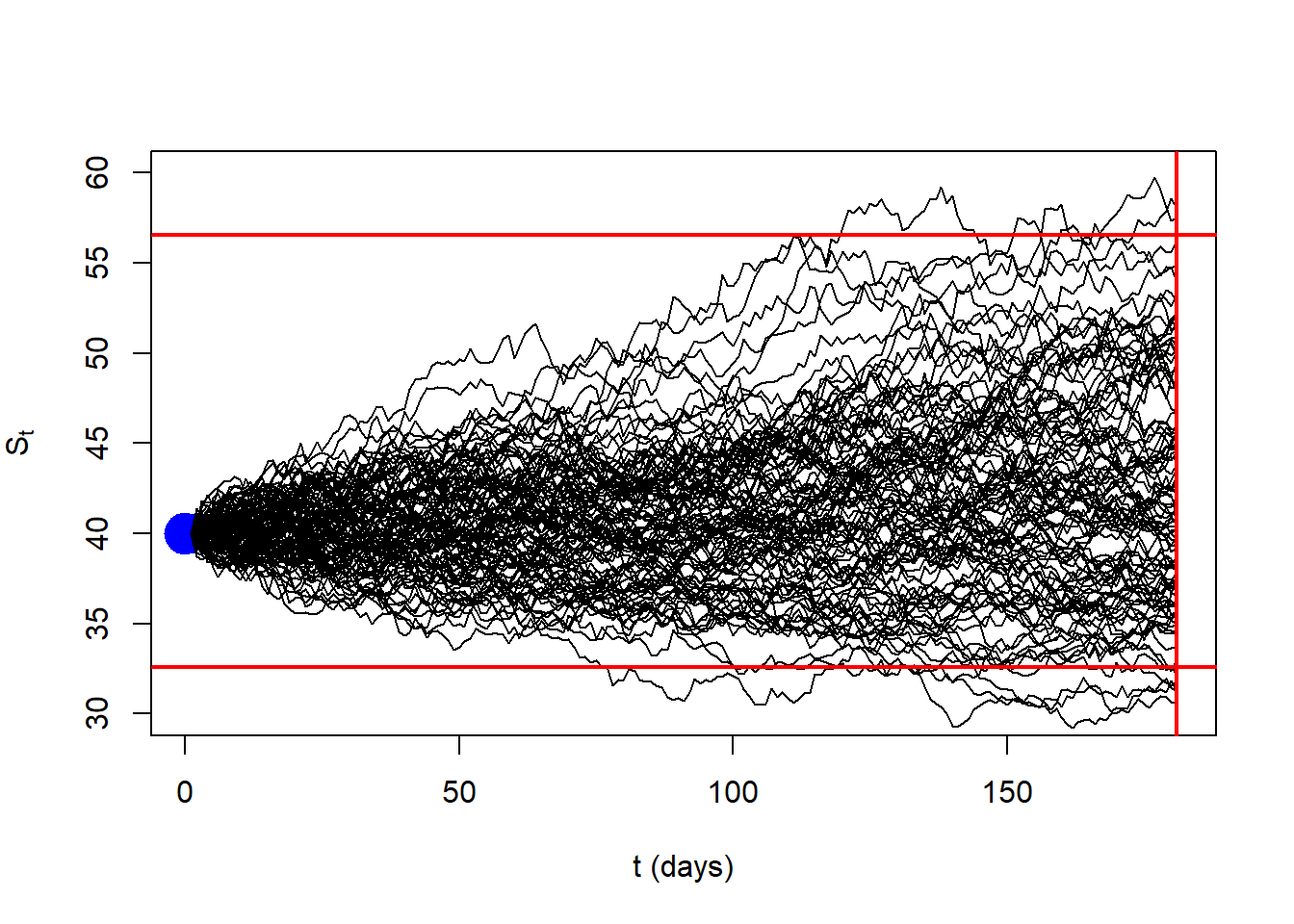

Figure 3.10: A geometric Brownian motion simulation: 100 stock price paths.

The code above can be problematic because we are not collecting all paths in an object. An alternative code is the following. Again, this is similar to example 15.1 in Hull (2015).

Code

S0 <- 40
nDays <- 360
mu <- 0.16
sig <- 0.2
TT <- 0.5
mean.logST <- log(S0)+(mu - (sig^2 / 2)) * TT
variance.logST <- sig^2 * TT
lower.ST <- exp(mean.logST + qnorm(0.025) * variance.logST^0.5)
upper.ST <- exp(mean.logST + qnorm(0.975) * variance.logST^0.5)
set.seed(3)
nSim <- 1000
nSteps <- nDays * TT
SP_sim <- matrix(0, nrow = nSteps + 1, ncol = nSim)
for(i in 1:nSim){
  SVec <- rep(0, nSteps + 1)
  SVec[1] <- S0
  for(j in 2:(nSteps + 1)){
    DeltaS <- mu * SVec[j - 1] * (1 / nDays) + sig * SVec[j - 1] *
      rnorm(1) * (1 / nDays)^0.5
    SVec[j] <- SVec[j - 1] + DeltaS
  }
  SP_sim[, i] <- SVec
}

Now, let’s plot the results.

Code

matplot(0:nSteps, SP_sim, type = 'l', col = rgb(0, 0, 1 ,0.3), lty = 1,
        ylab = expression(paste(S[t])),
        xlab = "Time")
points(0, S0, pch = 19, cex = 3)
abline(h = lower.ST)
abline(h = upper.ST)
abline(v = nSteps)

Figure 3.11: A geometric Brownian motion simulation: 1000 stock price paths.

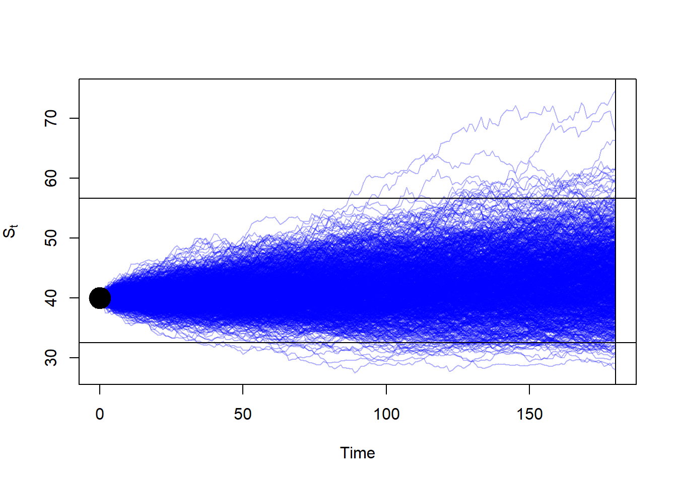
Let’s verify that there is approximately a 95% probability that the stock price in 6 months will lie between the lower and upper bounds shown above.

Code

1 - (sum(SP_sim[nSteps + 1, ] < lower.ST) + 
       sum(SP_sim[nSteps + 1, ] > upper.ST)) / 1000

[1] 0.967

Code

S0 <- 40
mu <- 0.16
sig <- 0.2
TT <- 0.5
mean.logST <- log(S0)+(mu - (sig^2 / 2)) * TT
variance.logST <- sig^2 * TT
lower.ST <- exp(mean.logST + qnorm(0.025) * variance.logST^0.5)
upper.ST <- exp(mean.logST + qnorm(0.975) * variance.logST^0.5)
lower.ST

[1] 32.51491

Code

upper.ST

[1] 56.6029

Nice.

This is how a stock price evolves according to the Black-Scholes formula.