2  Time series forecasting with machine learning in R

As in the previous chapter, the problem is to forecast one monthly time series: Beer, Wine, and Distilled Alcoholic Beverages Sales, following the original Matt Dancho example. The data comes from FRED, the Federal Reserve Economic Data database. The series belongs to the non-durable goods category; it includes U.S. merchant wholesalers, excluding manufacturers’ sales branches and offices. The observations run from 2010-01-01 to 2022-10-31. The goal is to estimate models with information available before 2022 and evaluate their forecasts over the 10 available months of 2022.

For the full database details see: https://fred.stlouisfed.org/series/S4248SM144NCEN

First load the R packages.

# Load libraries.
library(fpp3)
library(timetk)     # Toolkit for working with time series in R.
library(tidyquant)  # Loads tidyverse, financial packages, and data tools.
library(dplyr)      # Database manipulation.
library(ggplot2)    # Plots.
library(tibble)     # Tables.
library(kableExtra) # Tables.
library(knitr)
library(sweep)      # Broom-style tidiers for the forecast package.
library(forecast)   # Forecasting models and predictions package.
library(seasonal)
library(lubridate)
library(rpart)      # Lightweight regression trees.
library(nnet)       # Lightweight neural networks.

# This comes from 01-forecasting-with-fpp3.qmd.
mape_updated <- readRDS("mape_updated.rds")

We can conveniently download the data directly from the FRED API in one line of code.

# Beer, Wine, Distilled Alcoholic Beverages, in Millions USD.
beer <- tq_get("S4248SM144NCEN", get = "economic.data",
               from = "2010-01-01", to = "2022-10-31")

if (!is.data.frame(beer) || !all(c("date", "price") %in% names(beer))) {
  fred_beer <- read.csv(
    "https://fred.stlouisfed.org/graph/fredgraph.csv?id=S4248SM144NCEN",
    stringsAsFactors = FALSE
  )

  beer <- fred_beer %>%
    transmute(
      date = as.Date(observation_date),
      price = as.numeric(S4248SM144NCEN)
    ) %>%
    filter(date >= as.Date("2010-01-01"), date <= as.Date("2022-10-31")) %>%
    filter(!is.na(price))
}

if (!is.data.frame(beer) || !all(c("date", "price") %in% names(beer))) {
  stop("The FRED beer sales series could not be loaded as a data frame.")
}

The first rows show the structure of the data set. By default the value column is named price, although these are sales figures in monetary terms. According to the main FRED reference, these are in millions of dollars and are reported before seasonal adjustment.

head(beer)

# A tibble: 6 × 3
  symbol         date       price
  <chr>          <date>     <int>
1 S4248SM144NCEN 2010-01-01  6558
2 S4248SM144NCEN 2010-02-01  7481
3 S4248SM144NCEN 2010-03-01  9475
4 S4248SM144NCEN 2010-04-01  9424
5 S4248SM144NCEN 2010-05-01  9351
6 S4248SM144NCEN 2010-06-01 10552

We rename the value column so that the code matches the economic meaning of the variable.

beer <- beer %>%
  rename(sales = price)

tail(beer)

# A tibble: 6 × 3
  symbol         date       sales
  <chr>          <date>     <int>
1 S4248SM144NCEN 2022-05-01 16714
2 S4248SM144NCEN 2022-06-01 17899
3 S4248SM144NCEN 2022-07-01 15193
4 S4248SM144NCEN 2022-08-01 17069
5 S4248SM144NCEN 2022-09-01 16443
6 S4248SM144NCEN 2022-10-01 15585

The column name now identifies the variable as sales.

2.1 Supervised forecasting workflow

In this chapter, machine learning is used as a forecasting tool. The goal is narrowly defined: forecast a monthly time series by turning calendar and trend information into predictors. In time series forecasting, the supervised learning idea is to transform an ordered sequence into a modeling table: build a table of predictors called \(X\), keep the variable we want to forecast as \(y\), estimate a model on the training data, tune it with validation data, and evaluate it once on the test data.

This chapter uses the same forecasting problem as before with an explicit supervised forecasting workflow. The chapter writes the model comparison directly: we create the predictors, choose the candidate model families, tune the few hyperparameters by hand, and evaluate the final models on a holdout period. The models are smaller, faster to render in Quarto, easier to explain, and easier to debug. The workflow is also close to what students need to understand:

1. create time-based features;
2. split the data without shuffling the time order;
3. fit several explicit models;
4. choose hyperparameters with the validation set;
5. evaluate the chosen models on a test set held apart from fitting and tuning.

We will compare three transparent machine-learning forecasting alternatives:

• a multivariate linear regression;
• a regression tree;
• a small neural network.

The first model is highly interpretable. The tree is nonlinear and can capture simple threshold behavior. The neural network is also nonlinear. We keep it small so the model remains pedagogical and reproducible.

Mathematically, this chapter changes the forecasting problem from a univariate time-series model into a supervised forecasting regression problem. The first chapter used models built directly from the history of the series. This chapter turns each month into one row of a modeling table:

Row element	Meaning
sales	The value we want to forecast.
index.num	A numeric time trend.
year	A coarse trend variable and split variable.
month.lbl	Monthly seasonality.

Then each supervised forecasting model estimates a rule

\[ \text{sales} = f(\text{trend and month variables}) + \text{error}. \]

The three alternatives below differ in how flexible we allow the rule to be. Linear regression uses an additive straight-line rule. The regression tree uses if-then splits. The neural network uses a small nonlinear rule. The transparency principle is simple: we can see the columns, we can see the candidate model families, and the test set is reserved for the final evaluation.

The data split has three different jobs:

Sample	Dates	Job in the workflow
Training	2010-2020	Estimate model parameters.
Validation	2021	Choose hyperparameters such as tree complexity or neural-network size.
Test	January-October 2022	Evaluate the selected models once.

2.2 The data

We need an additional data set. The validation data set is used for model selection: it helps us choose hyperparameters before touching the final test period. The new data sets are the following.

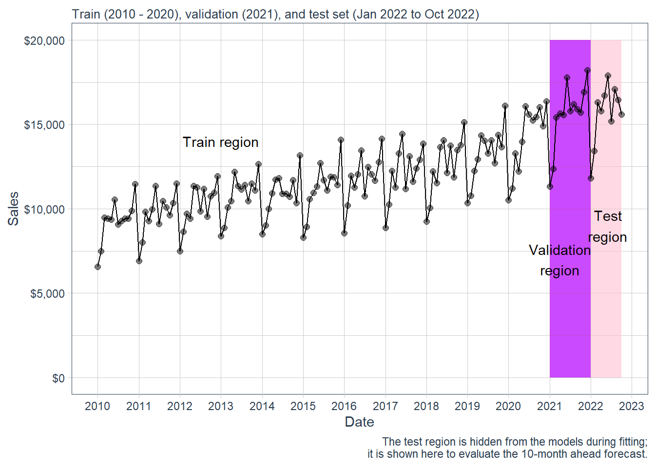
beer %>%
  ggplot(aes(date, sales)) +
  annotate("text", x = ymd("2013-01-01"), y = 14000,
           color = "black", label = "Train region") +
  geom_rect(xmin = as.numeric(ymd("2021-01-01")),
            xmax = as.numeric(ymd("2021-12-31")), ymin = 0, ymax = 20000,
            alpha = 0.01, fill = "purple") +
  annotate("text", x = ymd("2021-04-01"), y = 7000,
           color = "black", label = "Validation\nregion") +
  geom_rect(xmin = as.numeric(ymd("2022-01-01")),
            xmax = as.numeric(ymd("2022-09-30")), ymin = 0, ymax = 20000,
            alpha = 0.02, fill = "pink") +
  annotate("text", x = ymd("2022-06-01"), y = 9000,
           color = "black", label = "Test\nregion") +
  geom_line(col = "black") +
  geom_point(col = "black", alpha = 0.5, size = 2) +
  theme_tq() +
  scale_x_date(date_breaks = "1 year", date_labels = "%Y") +
  labs(subtitle =
  "Train (2010 - 2020), validation (2021), and test set (Jan 2022 to Oct 2022)",
  x = "Date", y = "Sales",
       caption = "The test region is hidden from the models during fitting;
       it is shown here to evaluate the 10-month ahead forecast.") +
  scale_y_continuous(labels = scales::dollar)

Figure 2.1: Beer sales: train, validation and test sets.

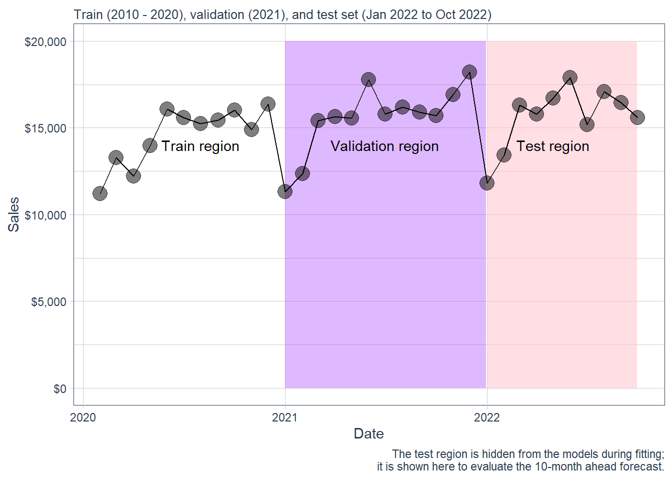
And the corresponding zoom version.

beer %>%
  filter(date > as.Date("2020-01-01")) %>%
  ggplot(aes(date, sales)) +
  annotate("text", x = ymd("2020-08-01"), y = 14000,
           color = "black", label = "Train region") +
  geom_rect(xmin = as.numeric(ymd("2021-01-01")),
            xmax = as.numeric(ymd("2021-12-31")), ymin = 0, ymax = 20000,
            alpha = 0.01, fill = "purple") +
  annotate("text", x = ymd("2021-07-01"), y = 14000,
           color = "black", label = "Validation region") +
  geom_rect(xmin = as.numeric(ymd("2022-01-01")),
            xmax = as.numeric(ymd("2022-09-30")), ymin = 0, ymax = 20000,
            alpha = 0.02, fill = "pink") +
  annotate("text", x = ymd("2022-05-01"), y = 14000,
           color = "black", label = "Test region") +
  geom_line(col = "black") +
  geom_point(col = "black", alpha = 0.5, size = 5) +
  theme_tq() +
  scale_x_date(date_breaks = "1 year", date_labels = "%Y") +
  labs(subtitle =
  "Train (2010 - 2020), validation (2021), and test set (Jan 2022 to Oct 2022)",
  x = "Date", y = "Sales",
       caption = "The test region is hidden from the models during fitting;
       it is shown here to evaluate the 10-month ahead forecast.") +
  scale_y_continuous(labels = scales::dollar)

Figure 2.2: Zoom. Beer sales: train, validation and test sets.

The tk_augment_timeseries_signature() function expands the timestamp information column-wise into a forecasting feature set. The original data set has a date, a symbol, and the sales variable. The augmented data includes calendar information such as year, month, quarter, semester and other time features. Only some of them will be useful for the final models. The full list still helps us inspect the forecasting problem as a supervised forecasting problem.

beer_aug <- beer %>%
  tk_augment_timeseries_signature()

tail(beer_aug)

# A tibble: 6 × 31
  symbol    date       sales index.num   diff  year year.iso  half quarter month
  <chr>     <date>     <int>     <dbl>  <dbl> <int>    <int> <int>   <int> <int>
1 S4248SM1… 2022-05-01 16714    1.65e9 2.59e6  2022     2022     1       2     5
2 S4248SM1… 2022-06-01 17899    1.65e9 2.68e6  2022     2022     1       2     6
3 S4248SM1… 2022-07-01 15193    1.66e9 2.59e6  2022     2022     2       3     7
4 S4248SM1… 2022-08-01 17069    1.66e9 2.68e6  2022     2022     2       3     8
5 S4248SM1… 2022-09-01 16443    1.66e9 2.68e6  2022     2022     2       3     9
6 S4248SM1… 2022-10-01 15585    1.66e9 2.59e6  2022     2022     2       4    10
# ℹ 21 more variables: month.xts <int>, month.lbl <ord>, day <int>, hour <int>,
#   minute <int>, second <int>, hour12 <int>, am.pm <int>, wday <int>,
#   wday.xts <int>, wday.lbl <ord>, mday <int>, qday <int>, yday <int>,
#   mweek <int>, week <int>, week.iso <int>, week2 <int>, week3 <int>,
#   week4 <int>, mday7 <int>

The variable names in beer_aug are:

colnames(beer_aug)

 [1] "symbol"    "date"      "sales"     "index.num" "diff"      "year"     
 [7] "year.iso"  "half"      "quarter"   "month"     "month.xts" "month.lbl"
[13] "day"       "hour"      "minute"    "second"    "hour12"    "am.pm"    
[19] "wday"      "wday.xts"  "wday.lbl"  "mday"      "qday"      "yday"     
[25] "mweek"     "week"      "week.iso"  "week2"     "week3"     "week4"    
[31] "mday7"    

The full signature is useful for inspection. For this monthly data set, it is broader than necessary. Many columns describe hours, seconds, weekdays, or day-of-month details. They are meaningful for hourly or daily data. In this monthly problem, they mostly encode calendar artifacts. We keep a smaller set:

• sales, the target variable;
• index.num, a numeric time index for the trend;
• year, a coarse trend variable that also makes the split readable;
• month.lbl, a factor for monthly seasonality.

This modeling decision keeps the target variable intact and makes the supervised forecasting matrix easier to explain. It also reduces dependence on irrelevant timestamp fragments.

The retained features define the design matrix used by the models. Because month.lbl is a categorical variable, R expands it internally into 0/1 dummy variables. For example, define

\[ D_{t,\text{Feb}} = \begin{cases} 1, & \text{month } t \text{ is February},\\ 0, & \text{otherwise.} \end{cases} \]

The same idea is repeated for March through December. Conceptually, the row for month \(t\) is

\[ x_t = \left[ 1,\, \text{index.num}_t,\, \text{year}_t,\, D_{t,\text{Feb}},\ldots, D_{t,\text{Dec}} \right]. \]

January is absorbed into the intercept by default. The important forecasting point is that every predictor in \(x_t\) is known before the sales value \(y_t\) is observed. Future dates, years, and months are known in advance, so these predictors keep the future sales value unavailable to the model.

selected_ml_columns <- c("sales", "index.num", "year", "month.lbl")

feature_decisions <- tibble(variable = colnames(beer_aug)) %>%
  mutate(
    decision = case_when(
      variable == "sales" ~ "Target",
      variable %in% selected_ml_columns ~ "Keep",
      TRUE ~ "Drop"
    ),
    reason = case_when(
      variable == "sales" ~ "Value we want to forecast.",
      variable == "index.num" ~ "Numeric trend over time.",
      variable == "year" ~ "Coarse trend and readable split variable.",
      variable == "month.lbl" ~ "Monthly seasonal factor.",
      variable == "date" ~ "Raw Date object; useful for plots; excluded as a direct predictor here.",
      variable == "symbol" ~ "Constant because there is only one series.",
      variable %in% c("hour", "minute", "second", "hour12", "am.pm") ~
        "Intraday information; irrelevant for monthly observations.",
      variable %in% c("day", "wday", "wday.xts", "wday.lbl", "mday",
                      "qday", "yday", "mweek", "week", "week.iso",
                      "week2", "week3", "week4", "mday7") ~
        "Daily or weekly calendar artifact for monthly data.",
      TRUE ~ "Redundant with the retained trend or monthly seasonality variables."
    )
  )

kable(feature_decisions,
      caption = "Feature-selection decision for the time-series signature.",
      row.names = FALSE) %>%
  kable_styling(latex_options = "HOLD_position")

Feature-selection decision for the time-series signature.

variable	decision	reason
symbol	Drop	Constant because there is only one series.
date	Drop	Raw Date object; useful for plots; excluded as a direct predictor here.
sales	Target	Value we want to forecast.
index.num	Keep	Numeric trend over time.
diff	Drop	Redundant with the retained trend or monthly seasonality variables.
year	Keep	Coarse trend and readable split variable.
year.iso	Drop	Redundant with the retained trend or monthly seasonality variables.
half	Drop	Redundant with the retained trend or monthly seasonality variables.
quarter	Drop	Redundant with the retained trend or monthly seasonality variables.
month	Drop	Redundant with the retained trend or monthly seasonality variables.
month.xts	Drop	Redundant with the retained trend or monthly seasonality variables.
month.lbl	Keep	Monthly seasonal factor.
day	Drop	Daily or weekly calendar artifact for monthly data.
hour	Drop	Intraday information; irrelevant for monthly observations.
minute	Drop	Intraday information; irrelevant for monthly observations.
second	Drop	Intraday information; irrelevant for monthly observations.
hour12	Drop	Intraday information; irrelevant for monthly observations.
am.pm	Drop	Intraday information; irrelevant for monthly observations.
wday	Drop	Daily or weekly calendar artifact for monthly data.
wday.xts	Drop	Daily or weekly calendar artifact for monthly data.
wday.lbl	Drop	Daily or weekly calendar artifact for monthly data.
mday	Drop	Daily or weekly calendar artifact for monthly data.
qday	Drop	Daily or weekly calendar artifact for monthly data.
yday	Drop	Daily or weekly calendar artifact for monthly data.
mweek	Drop	Daily or weekly calendar artifact for monthly data.
week	Drop	Daily or weekly calendar artifact for monthly data.
week.iso	Drop	Daily or weekly calendar artifact for monthly data.
week2	Drop	Daily or weekly calendar artifact for monthly data.
week3	Drop	Daily or weekly calendar artifact for monthly data.
week4	Drop	Daily or weekly calendar artifact for monthly data.
mday7	Drop	Daily or weekly calendar artifact for monthly data.

We now build the actual modeling table from the selected variables and convert ordered factors into plain factors. The target variable sales remains unchanged; the code only prepares the predictor matrix.

beer_clean <- beer_aug %>%
  select(all_of(selected_ml_columns)) %>%
  mutate_if(is.ordered, ~ as.character(.) %>% as.factor)

head(beer_clean)

# A tibble: 6 × 4
  sales  index.num  year month.lbl
  <int>      <dbl> <int> <fct>    
1  6558 1262304000  2010 enero    
2  7481 1264982400  2010 febrero  
3  9475 1267401600  2010 marzo    
4  9424 1270080000  2010 abril    
5  9351 1272672000  2010 mayo     
6 10552 1275350400  2010 junio    

We split the database into training, validation and test sets following the time ranges in the visualization above. The test set is the most recent data. It remains unavailable during model fitting and tuning.

The split can be read directly from the year column:

Sample	Rule in the code	Use
Training	year < 2021	Fit model parameters.
Validation	year == 2021	Choose hyperparameters.
Test	year == 2022	Evaluate the chosen models.

The validation set is used to choose hyperparameters. The test set is used only after the choices have been made.

train_tbl <- beer_clean %>% filter(year < 2021)
valid_tbl <- beer_clean %>% filter(year == 2021)
test_tbl  <- beer_clean %>% filter(year == 2022)

test_tbl$sales

 [1] 11801 13435 16292 15772 16714 17899 15193 17069 16443 15585

Our goal is to forecast the first 10 months of 2022.

2.3 Validation workflow

The following support functions keep the comparison compact. They calculate the same error measures for every model: mean error, root mean squared error, mean absolute error, mean absolute percentage error, and mean percentage error.

For a validation or test sample of size \(n\), with predictions \(\hat{y}_t\), the main metrics are:

\[ \text{ME} = \frac{1}{n}\sum_{t=1}^{n}(y_t-\hat{y}_t), \]

\[ \text{RMSE} = \sqrt{\frac{1}{n}\sum_{t=1}^{n}(y_t-\hat{y}_t)^2}, \]

\[ \text{MAE} = \frac{1}{n}\sum_{t=1}^{n}|y_t-\hat{y}_t|, \]

\[ \text{MAPE} = \frac{100}{n}\sum_{t=1}^{n} \left| \frac{y_t-\hat{y}_t}{y_t} \right|. \]

The code below implements these formulas directly. This keeps the workflow auditable because the evaluation formulas are visible in the chapter.

metric_tbl <- function(actual, pred) {
  residuals <- actual - pred
  pct_error <- residuals / actual

  tibble(
    me = mean(residuals, na.rm = TRUE),
    rmse = sqrt(mean(residuals^2, na.rm = TRUE)),
    mae = mean(abs(residuals), na.rm = TRUE),
    mape = 100 * mean(abs(pct_error), na.rm = TRUE),
    mpe = 100 * mean(pct_error, na.rm = TRUE)
  )
}

validation_row <- function(model, family, setting, actual, pred) {
  bind_cols(
    tibble(model = model, family = family, setting = setting),
    metric_tbl(actual, pred)
  )
}

forecast_error_tbl <- function(model, pred) {
  beer %>%
    filter(lubridate::year(date) == 2022) %>%
    transmute(
      model = model,
      date = date,
      actual = sales,
      pred = as.numeric(pred),
      error = actual - pred,
      error_pct = error / actual
    )
}

The linear regression has no hyperparameters. It is our transparent baseline. If this model works well, that is useful information: sometimes a simple model is enough when trend and seasonality are strong.

The fitted linear regression equation is

\[ y_t = \beta_0 + \beta_1\,\text{index.num}_t + \beta_2\,\text{year}_t + \sum_{j=2}^{12}\gamma_j D_{t,j} + \varepsilon_t. \]

Here, \(D_{t,j}\) is a monthly dummy variable: it equals 1 when observation \(t\) belongs to month \(j\), and 0 otherwise. January is the baseline month because it is absorbed by the intercept. The coefficients have a direct interpretation: the trend variables explain long-run movement, and the monthly dummy variables explain seasonality relative to January. The code lm(sales ~ .) means: regress sales on all remaining columns in the modeling table.

ml_formula <- sales ~ .

fit_lm_valid <- lm(ml_formula, data = train_tbl)
pred_lm_valid <- as.numeric(predict(fit_lm_valid, newdata = valid_tbl))

lm_validation <- validation_row(
  model = "Linear regression",
  family = "Linear regression",
  setting = "selected calendar features",
  actual = valid_tbl$sales,
  pred = pred_lm_valid
)

The regression tree has a complexity parameter, cp. A smaller value allows a larger tree; a larger value prunes the tree more aggressively. We estimate a small grid and choose the value that minimizes validation RMSE.

A regression tree asks a sequence of yes/no questions about the predictors. For example: is the month December? is the time index above a certain value? After following those questions to a final group, the forecast is the average sales value among the training observations in that group:

\[ \text{tree forecast} = \text{average sales in the final group}. \]

The cp parameter controls the cost of adding more splits. A useful way to read it is as a penalty on tree complexity: larger cp values prune more splits, and smaller cp values allow more splits.

Small cp values allow more regions and can overfit. Large cp values produce simpler trees and can underfit. We choose cp using the validation set. The test set remains reserved for the final evaluation.

tree_grid <- tibble(cp = c(0.001, 0.005, 0.01, 0.02, 0.05))

tree_validation <- bind_rows(lapply(seq_len(nrow(tree_grid)), function(i) {
  fit_tree <- rpart::rpart(
    ml_formula,
    data = train_tbl,
    method = "anova",
    control = rpart::rpart.control(
      cp = tree_grid$cp[i],
      minsplit = 8,
      xval = 0
    )
  )

  pred_tree <- as.numeric(predict(fit_tree, newdata = valid_tbl))

  validation_row(
    model = "Regression tree",
    family = "Regression tree",
    setting = paste0("cp = ", tree_grid$cp[i]),
    actual = valid_tbl$sales,
    pred = pred_tree
  )
}))

best_tree <- tree_validation %>%
  arrange(rmse) %>%
  slice(1)

The neural network also receives a small manual search. We tune two hyperparameters: size, the number of hidden units, and decay, a penalty that discourages overly large weights. Because the variables have different scales, we standardize the model matrix before fitting.

The neural network uses the same predictors as the linear regression and tree. The difference is the way it combines them. It first standardizes the inputs, then creates a small number of hidden units, and finally combines those hidden units into one forecast. The size hyperparameter controls how many hidden units are used. The decay hyperparameter discourages very large weights, so the fitted rule stays smoother.

Its inputs remain the same explicit features used by the linear regression and the tree. The extra flexibility comes from the hidden layer and the nonlinear activation function.

The support functions below do five mechanical tasks:

Step	What the code does	Why it is important
1	Build the model matrix from the formula.	Convert factors such as month into numeric columns.
2	Standardize the predictors.	Put all inputs on comparable scales.
3	Standardize the target variable.	Help the neural network optimize more smoothly.
4	Fit the network with nnet().	Estimate the weights in the hidden and output layers.
5	Undo the scaling during prediction.	Return forecasts in the original sales units.

fit_nnet_regression <- function(train_data, size, decay, seed = 13) {
  x <- model.matrix(ml_formula, data = train_data)[, -1, drop = FALSE]

  center <- apply(x, 2, mean)
  scale <- apply(x, 2, sd)
  scale[is.na(scale) | scale == 0] <- 1

  x_scaled <- sweep(sweep(x, 2, center, "-"), 2, scale, "/")

  y_center <- mean(train_data$sales)
  y_scale <- sd(train_data$sales)
  if (is.na(y_scale) || y_scale == 0) y_scale <- 1

  set.seed(seed)
  fit <- nnet::nnet(
    x = x_scaled,
    y = (train_data$sales - y_center) / y_scale,
    size = size,
    decay = decay,
    linout = TRUE,
    trace = FALSE,
    maxit = 1000
  )

  list(
    fit = fit,
    columns = colnames(x),
    center = center,
    scale = scale,
    y_center = y_center,
    y_scale = y_scale
  )
}

predict_nnet_regression <- function(object, new_data) {
  x <- model.matrix(ml_formula, data = new_data)[, -1, drop = FALSE]

  missing_cols <- setdiff(object$columns, colnames(x))
  if (length(missing_cols) > 0) {
    missing_matrix <- matrix(0, nrow = nrow(x), ncol = length(missing_cols))
    colnames(missing_matrix) <- missing_cols
    x <- cbind(x, missing_matrix)
  }

  x <- x[, object$columns, drop = FALSE]
  x_scaled <- sweep(sweep(x, 2, object$center, "-"), 2, object$scale, "/")

  as.numeric(predict(object$fit, x_scaled)) * object$y_scale + object$y_center
}

nnet_grid <- expand.grid(
  size = c(1, 3, 5),
  decay = c(0, 0.001, 0.01)
)

nnet_validation <- bind_rows(lapply(seq_len(nrow(nnet_grid)), function(i) {
  fit_nnet <- fit_nnet_regression(
    train_data = train_tbl,
    size = nnet_grid$size[i],
    decay = nnet_grid$decay[i],
    seed = 13 + i
  )

  pred_nnet <- predict_nnet_regression(fit_nnet, valid_tbl)

  validation_row(
    model = "Neural network",
    family = "Neural network",
    setting = paste0("size = ", nnet_grid$size[i],
                     ", decay = ", nnet_grid$decay[i]),
    actual = valid_tbl$sales,
    pred = pred_nnet
  )
}))

best_nnet <- nnet_validation %>%
  arrange(rmse) %>%
  slice(1)

The validation leaderboard summarizes the model selection step. The final forecasting performance is evaluated later with the test set.

For each model family, we choose the setting with the smallest validation RMSE. For the tree, the setting is cp. For the neural network, the setting is the pair (size, decay). Linear regression has no tuning grid, so it enters the leaderboard once.

validation_leaderboard <- bind_rows(
  lm_validation,
  tree_validation,
  nnet_validation
) %>%
  arrange(rmse)

kable(validation_leaderboard,
      caption = "Validation leaderboard for machine-learning forecasting models.",
      digits = 2) %>%
  kable_styling(latex_options = "HOLD_position")

Validation leaderboard for machine-learning forecasting models.

model	family	setting	me	rmse	mae	mape	mpe
Neural network	Neural network	size = 3, decay = 0	488.20	1138.07	836.93	5.63	2.87
Neural network	Neural network	size = 3, decay = 0.01	792.02	1179.28	954.10	5.94	4.90
Neural network	Neural network	size = 1, decay = 0	1060.20	1195.32	1060.20	6.72	6.72
Neural network	Neural network	size = 1, decay = 0.001	1150.18	1266.56	1150.18	7.30	7.30
Neural network	Neural network	size = 5, decay = 0.01	794.89	1313.70	1087.58	6.97	5.10
Neural network	Neural network	size = 1, decay = 0.01	1236.29	1346.37	1236.29	7.81	7.81
Neural network	Neural network	size = 5, decay = 0	392.53	1370.39	1185.47	7.59	2.22
Neural network	Neural network	size = 3, decay = 0.001	1098.68	1410.56	1149.21	7.10	6.66
Linear regression	Linear regression	selected calendar features	1367.15	1550.66	1372.10	8.40	8.36
Neural network	Neural network	size = 5, decay = 0.001	-92.34	1640.64	1223.46	7.69	-0.80
Regression tree	Regression tree	cp = 0.001	1352.94	1788.57	1382.30	8.78	8.60
Regression tree	Regression tree	cp = 0.005	1445.38	1859.65	1474.74	9.57	9.38
Regression tree	Regression tree	cp = 0.01	1445.38	1859.65	1474.74	9.57	9.38
Regression tree	Regression tree	cp = 0.02	1400.90	1948.70	1400.90	8.83	8.83
Regression tree	Regression tree	cp = 0.05	1400.90	1948.70	1400.90	8.83	8.83

2.4 Test forecasts

Now we refit the chosen model specifications using the training and validation data together, from 2010 through 2021. Then we forecast the 2022 test set. This is a standard practice: validation is used to make modeling decisions, and after that decision is made we can use all pre-test information to estimate the final model.

The final fitted function uses all observations from 2010 through 2021 and the hyperparameters selected in validation. The test forecasts are obtained by applying that final fitted rule to the 2022 rows.

This ordering prevents methodological leakage: the test sales values never enter coefficient estimation, cp selection, neural-network size selection, or neural-network decay selection.

train_valid_tbl <- beer_clean %>%
  filter(year < 2022)

fit_lm_final <- lm(ml_formula, data = train_valid_tbl)
pred_lm_test <- as.numeric(predict(fit_lm_final, newdata = test_tbl))

fit_tree_final <- rpart::rpart(
  ml_formula,
  data = train_valid_tbl,
  method = "anova",
  control = rpart::rpart.control(
    cp = best_tree$setting %>%
      sub("cp = ", "", .) %>%
      as.numeric(),
    minsplit = 8,
    xval = 0
  )
)
pred_tree_test <- as.numeric(predict(fit_tree_final, newdata = test_tbl))

best_nnet_size <- sub("size = ([0-9]+),.*", "\\1", best_nnet$setting) %>%
  as.numeric()
best_nnet_decay <- sub(".*decay = ([0-9.]+)", "\\1", best_nnet$setting) %>%
  as.numeric()

fit_nnet_final <- fit_nnet_regression(
  train_data = train_valid_tbl,
  size = best_nnet_size,
  decay = best_nnet_decay,
  seed = 100
)
pred_nnet_test <- predict_nnet_regression(fit_nnet_final, test_tbl)

The table below shows the 10-month forecast errors.

ml_errors <- bind_rows(
  forecast_error_tbl("ML forecast: linear regression", pred_lm_test),
  forecast_error_tbl("ML forecast: regression tree", pred_tree_test),
  forecast_error_tbl("ML forecast: neural network", pred_nnet_test)
)

kable(ml_errors,
      caption = "Detailed test performance for machine-learning forecasting models.",
      digits = 3,
      row.names = FALSE) %>%
  kable_styling(latex_options = "HOLD_position")

Detailed test performance for machine-learning forecasting models.

model	date	actual	pred	error	error_pct
ML forecast: linear regression	2022-01-01	11801	12048.17	-247.168	-0.021
ML forecast: linear regression	2022-02-01	13435	12948.50	486.498	0.036
ML forecast: linear regression	2022-03-01	16292	14619.16	1672.844	0.103
ML forecast: linear regression	2022-04-01	15772	14477.24	1294.761	0.082
ML forecast: linear regression	2022-05-01	16714	15601.41	1112.594	0.067
ML forecast: linear regression	2022-06-01	17899	16443.74	1455.261	0.081
ML forecast: linear regression	2022-07-01	15193	14908.49	284.511	0.019
ML forecast: linear regression	2022-08-01	17069	15625.41	1443.594	0.085
ML forecast: linear regression	2022-09-01	16443	15013.07	1429.927	0.087
ML forecast: linear regression	2022-10-01	15585	15577.07	7.927	0.001
ML forecast: regression tree	2022-01-01	11801	11084.83	716.167	0.061
ML forecast: regression tree	2022-02-01	13435	11084.83	2350.167	0.175
ML forecast: regression tree	2022-03-01	16292	16173.25	118.750	0.007
ML forecast: regression tree	2022-04-01	15772	16173.25	-401.250	-0.025
ML forecast: regression tree	2022-05-01	16714	16173.25	540.750	0.032
ML forecast: regression tree	2022-06-01	17899	17100.25	798.750	0.045
ML forecast: regression tree	2022-07-01	15193	16173.25	-980.250	-0.065
ML forecast: regression tree	2022-08-01	17069	16173.25	895.750	0.052
ML forecast: regression tree	2022-09-01	16443	16173.25	269.750	0.016
ML forecast: regression tree	2022-10-01	15585	16173.25	-588.250	-0.038
ML forecast: neural network	2022-01-01	11801	11289.04	511.964	0.043
ML forecast: neural network	2022-02-01	13435	12925.93	509.073	0.038
ML forecast: neural network	2022-03-01	16292	16326.27	-34.270	-0.002
ML forecast: neural network	2022-04-01	15772	16363.52	-591.524	-0.038
ML forecast: neural network	2022-05-01	16714	16184.65	529.346	0.032
ML forecast: neural network	2022-06-01	17899	17725.16	173.840	0.010
ML forecast: neural network	2022-07-01	15193	17594.15	-2401.155	-0.158
ML forecast: neural network	2022-08-01	17069	16734.07	334.930	0.020
ML forecast: neural network	2022-09-01	16443	17511.51	-1068.509	-0.065
ML forecast: neural network	2022-10-01	15585	16931.42	-1346.422	-0.086

The same information is clearer in a plot. The black line is the actual series. The colored lines are the machine-learning forecasts for the 2022 test period.

beer %>%
  filter(date > as.Date("2021-01-01")) %>%
  ggplot(aes(x = yearmonth(date), y = sales)) +
  geom_line(color = "black", linewidth = 0.5) +
  geom_point(color = "black", size = 4, alpha = 0.5) +
  geom_line(aes(y = pred, color = model), linewidth = 0.7,
            data = ml_errors) +
  geom_point(aes(y = pred, color = model), size = 3, alpha = 0.8,
             data = ml_errors) +
  geom_vline(xintercept = as.numeric(as.Date("2021-12-01")), linetype = 2) +
  theme_tq() +
  labs(x = "Date", y = "Sales", color = "Model") +
  scale_y_continuous(labels = scales::dollar)

Figure 2.3: Forecasts from machine-learning forecasting models.

The overall test summary is:

ml_summary <- ml_errors %>%
  group_by(model) %>%
  summarise(
    me = mean(error),
    rmse = sqrt(mean(error^2)),
    mae = mean(abs(error)),
    mape = 100 * mean(abs(error_pct)),
    mpe = 100 * mean(error_pct),
    .groups = "drop"
  ) %>%
  arrange(mape)

kable(ml_summary,
      caption = "Test summary for machine-learning forecasting models.",
      digits = 2) %>%
  kable_styling(latex_options = "HOLD_position")

Test summary for machine-learning forecasting models.

model	me	rmse	mae	mape	mpe
ML forecast: neural network	-338.27	1000.75	750.10	4.91	-2.07
ML forecast: regression tree	372.03	965.60	765.98	5.16	2.61
ML forecast: linear regression	894.07	1110.76	943.51	5.81	5.39

A model can rank first by MAPE and rank differently by another metric. For that reason, it is useful to inspect multiple errors. RMSE penalizes large mistakes more heavily, while MAPE is easy to read as an average percentage error.

The table compares fitted forecasting functions under a common experimental design. Every model saw the same training data, the same validation data, the same predictors, and the same test months. A lower MAPE means that this particular fitted function was closer to the realized 2022 sales over this holdout period.

In the current render, the machine-learning neural network forecast is the best of the three supervised forecasting models, with MAPE around 4.91. The regression tree follows with MAPE around 5.16, and the linear regression has MAPE around 5.81. The differences are modest, so the interpretation should focus on the pattern: calendar and trend predictors carry useful information, and a small nonlinear model extracts a little more from those predictors in this test window.

We can also show the best individual point forecast for each model.

point_forecast_ml <- ml_errors %>%
  group_by(model) %>%
  slice_min(abs(error_pct), n = 1, with_ties = FALSE) %>%
  ungroup() %>%
  select(model, date, actual, pred, error, error_pct)

kable(point_forecast_ml,
      caption = "Best point forecast for each machine-learning forecasting model.",
      digits = 4,
      row.names = FALSE) %>%
  kable_styling(latex_options = "HOLD_position")

Best point forecast for each machine-learning forecasting model.

model	date	actual	pred	error	error_pct
ML forecast: linear regression	2022-10-01	15585	15577.07	7.9273	0.0005
ML forecast: neural network	2022-03-01	16292	16326.27	-34.2696	-0.0021
ML forecast: regression tree	2022-03-01	16292	16173.25	118.7500	0.0073

Choosing a model according to one specific point forecast would be fragile. Even so, it is useful to see where each model was most accurate.

mape_updated_ml <- mape_updated %>%
  add_row(.model = "ML forecast: linear regression",
          MAPE = ml_summary$mape[ml_summary$model == "ML forecast: linear regression"]) %>%
  add_row(.model = "ML forecast: regression tree",
          MAPE = ml_summary$mape[ml_summary$model == "ML forecast: regression tree"]) %>%
  add_row(.model = "ML forecast: neural network",
          MAPE = ml_summary$mape[ml_summary$model == "ML forecast: neural network"]) %>%
  arrange(MAPE)

mape_updated_ml

# A tibble: 10 × 2
   .model                          MAPE
   <chr>                          <dbl>
 1 fpp3: ETS(M,A,M)                3.77
 2 fpp3: seasonal naïve            3.89
 3 fpp3: ARIMA(4,1,1)(0,1,1)[12]   4.40
 4 ML forecast: neural network     4.91
 5 ML forecast: regression tree    5.16
 6 ML forecast: linear regression  5.81
 7 fpp3: NNAR(15,1,8)[12]          6.02
 8 fpp3: naïve                    18.1 
 9 fpp3: drift                    20.9 
10 fpp3: mean                     23.5 

2.5 ARIMA comparison

As in the original Matt Dancho example, we include a different ARIMA workflow using the forecast package and the auto.arima() function. This benchmark belongs to the classical time-series family and answers a different modeling question. The machine-learning forecasting models above estimate \(\text{sales}=f(\text{trend and month variables})+\text{error}\) using trend and calendar predictors. ARIMA models the dependence of the series on its own past.

The auto.arima() function automates the selection of the ARIMA orders. The automation is a statistical search over candidate values of \((p,d,q)(P,D,Q)_{12}\), followed by parameter estimation and information-criterion comparison.

The order notation is read as follows:

Order	Meaning
\(p\)	Number of recent lagged values used by the autoregressive part.
\(d\)	Number of ordinary differences.
\(q\)	Number of recent forecast errors used by the moving-average part.
\(P\)	Number of seasonal lagged values.
\(D\)	Number of seasonal differences.
\(Q\)	Number of seasonal forecast errors.
12	Monthly seasonal cycle.

Prepare the data.

The tk_ts() function coerces time series objects and tibbles with date or date-time columns to ts.

beer_sales_ts <- tk_ts(
  beer %>% filter(date < as.Date("2022-01-01")),
  start = 2010,
  freq = 12
)
beer_sales_ts

       Jan   Feb   Mar   Apr   May   Jun   Jul   Aug   Sep   Oct   Nov   Dec
2010  6558  7481  9475  9424  9351 10552  9077  9273  9420  9413  9866 11455
2011  6901  8014  9832  9281  9967 11344  9106 10469 10085  9612 10328 11483
2012  7486  8641  9709  9423 11342 11274  9845 11163  9532 10754 10953 11922
2013  8384  8871 10085 10462 12177 11342 11139 11408 10441 11480 11077 12635
2014  8505  9003  9991 10903 11709 11814 10875 10885 10725 11698 10353 13153
2015  8279  8926 10557 10934 11330 12709 11700 11078 11882 11865 11420 14099
2016  8555 10197 11948 11253 12046 13454 10755 12465 12038 11674 12762 14139
2017  8872 10255 12245 11270 13279 14432 11166 13099 11616 12382 12897 13849
2018  9235 10040 12205 11514 13653 14054 12125 13732 11874 13478 13759 15135
2019 10353 10764 12228 12922 14347 14033 13275 14047 12715 14386 13645 16110
2020 10521 11201 13281 12225 13977 16065 15577 15225 15446 16024 14890 16353
2021 11305 12365 15404 15646 15569 17782 15792 16191 15913 15689 16900 18201

Just verify that the tk_ts() function worked.

has_timetk_idx(beer_sales_ts)

[1] TRUE

Estimation.

We can use the auto.arima() function from the forecast package to model the time series. The function tests a set of specifications and selects the one that performs best according to its internal statistical criterion.

set.seed(13)
fit_arima <- auto.arima(beer_sales_ts)
fit_arima

Series: beer_sales_ts 
ARIMA(1,1,2)(2,1,1)[12] 

Coefficients:
          ar1     ma1      ma2    sar1     sar2     sma1
      -0.7375  0.1006  -0.7161  0.4054  -0.3543  -0.8232
s.e.   0.0978  0.0885   0.0719  0.1107   0.1043   0.1315

sigma^2 = 293810:  log likelihood = -1015.95
AIC=2045.9   AICc=2046.81   BIC=2066.02

The printed output is the selected mathematical specification. After this line, we are no longer speaking abstractly about auto.arima(); we are speaking about the particular ARIMA equation selected for this data set and this training window.

The sw_tidy() function returns the model coefficients in a tibble.

sw_tidy(fit_arima)

# A tibble: 6 × 2
  term  estimate
  <chr>    <dbl>
1 ar1     -0.738
2 ma1      0.101
3 ma2     -0.716
4 sar1     0.405
5 sar2    -0.354
6 sma1    -0.823

The sw_glance() function returns training-set accuracy measures.

sw_glance(fit_arima) %>%
  glimpse()

Rows: 1
Columns: 12
$ model.desc <chr> "ARIMA(1,1,2)(2,1,1)[12]"
$ sigma      <dbl> 542.0421
$ logLik     <dbl> -1015.948
$ AIC        <dbl> 2045.895
$ BIC        <dbl> 2066.022
$ ME         <dbl> 44.83642
$ RMSE       <dbl> 505.0179
$ MAE        <dbl> 374.7736
$ MPE        <dbl> 0.1094178
$ MAPE       <dbl> 3.074036
$ MASE       <dbl> 0.5452094
$ ACF1       <dbl> -0.0315898

Forecast.

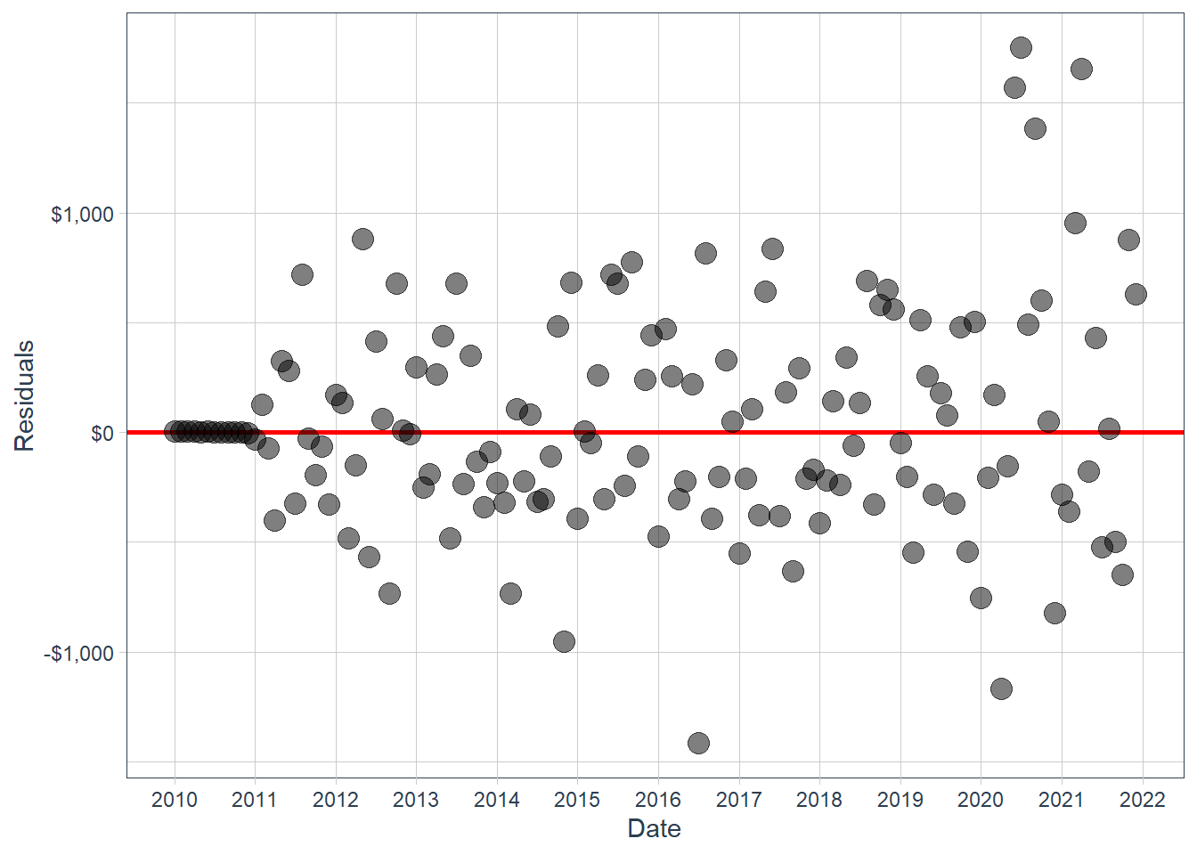
The sw_augment() function helps with model evaluation. We get the .actual, .fitted and .resid columns, which are useful in evaluating the model against the training data.

sw_augment(fit_arima, timetk_idx = TRUE)

# A tibble: 144 × 4
   index      .actual .fitted .resid
   <date>       <dbl>   <dbl>  <dbl>
 1 2010-01-01    6558   6554.  3.79 
 2 2010-02-01    7481   7479.  2.41 
 3 2010-03-01    9475   9472.  3.26 
 4 2010-04-01    9424   9422.  2.39 
 5 2010-05-01    9351   9349.  1.84 
 6 2010-06-01   10552  10549.  2.63 
 7 2010-07-01    9077   9076.  0.882
 8 2010-08-01    9273   9272.  0.956
 9 2010-09-01    9420   9419.  0.988
10 2010-10-01    9413   9412.  0.882
# ℹ 134 more rows

We can visualize the residual diagnostics for the training data.

sw_augment(fit_arima, timetk_idx = TRUE) %>%
  ggplot(aes(x = index, y = .resid)) +
  geom_hline(yintercept = 0, color = "red", linewidth = 1) +
  geom_point(size = 4, alpha = 0.5) +
  labs(x = "Date", y = "Residuals") +
  scale_x_date(date_breaks = "1 year", date_labels = "%Y") +
  theme_tq() +
  scale_y_continuous(labels = scales::dollar)

Figure 2.4: forecast::auto.arima residual diagnosis.

The residuals are

\[ \hat{\varepsilon}_t = y_t - \hat{y}_{t\mid t-1}. \]

If the ARIMA model has captured the predictable autocorrelation, these residuals should have no obvious remaining time pattern. This is the same audit logic used in the fpp3 chapter.

Make a forecast using the forecast() function.

fcast_arima <- forecast(fit_arima, h = 10)
fcast_arima

         Point Forecast    Lo 80    Hi 80    Lo 95    Hi 95
Jan 2022       12958.70 12262.28 13655.11 11893.62 14023.77
Feb 2022       13978.00 13237.17 14718.84 12844.99 15111.01
Mar 2022       16341.49 15596.23 17086.75 15201.71 17481.27
Apr 2022       16704.29 15930.63 17477.96 15521.07 17887.52
May 2022       17095.58 16313.50 17877.65 15899.50 18291.66
Jun 2022       18163.88 17360.62 18967.14 16935.40 19392.36
Jul 2022       16011.91 15197.81 16826.02 14766.85 17256.98
Aug 2022       16996.29 16164.63 17827.95 15724.38 18268.21
Sep 2022       16153.24 15309.50 16996.97 14862.86 17443.61
Oct 2022       16437.31 15578.01 17296.60 15123.13 17751.48

We use sw_sweep() to tidy the forecast output.

fcast_tbl <- sw_sweep(fcast_arima, timetk_idx = TRUE)
tail(fcast_tbl, 10)

# A tibble: 10 × 7
   index      key       sales  lo.80  lo.95  hi.80  hi.95
   <date>     <chr>     <dbl>  <dbl>  <dbl>  <dbl>  <dbl>
 1 2022-01-01 forecast 12959. 12262. 11894. 13655. 14024.
 2 2022-02-01 forecast 13978. 13237. 12845. 14719. 15111.
 3 2022-03-01 forecast 16341. 15596. 15202. 17087. 17481.
 4 2022-04-01 forecast 16704. 15931. 15521. 17478. 17888.
 5 2022-05-01 forecast 17096. 16314. 15899. 17878. 18292.
 6 2022-06-01 forecast 18164. 17361. 16935. 18967. 19392.
 7 2022-07-01 forecast 16012. 15198. 14767. 16826. 17257.
 8 2022-08-01 forecast 16996. 16165. 15724. 17828. 18268.
 9 2022-09-01 forecast 16153. 15310. 14863. 16997. 17444.
10 2022-10-01 forecast 16437. 15578. 15123. 17297. 17751.

We can investigate the error on our test set.

actuals_tbl <- beer %>%
  filter(lubridate::year(date) == 2022) %>%
  select(date, sales)

error_tbl_arima <- left_join(actuals_tbl, fcast_tbl,
                             by = c("date" = "index")) %>%
  rename(actual = sales.x, pred = sales.y) %>%
  select(date, actual, pred) %>%
  mutate(error = round((actual - pred), 2),
         error_pct = round((error / actual), 4))

error_tbl_arima

# A tibble: 10 × 5
   date       actual   pred   error error_pct
   <date>      <int>  <dbl>   <dbl>     <dbl>
 1 2022-01-01  11801 12959. -1158.    -0.0981
 2 2022-02-01  13435 13978.  -543     -0.0404
 3 2022-03-01  16292 16341.   -49.5   -0.003 
 4 2022-04-01  15772 16704.  -932.    -0.0591
 5 2022-05-01  16714 17096.  -382.    -0.0228
 6 2022-06-01  17899 18164.  -265.    -0.0148
 7 2022-07-01  15193 16012.  -819.    -0.0539
 8 2022-08-01  17069 16996.    72.7    0.0043
 9 2022-09-01  16443 16153.   290.     0.0176
10 2022-10-01  15585 16437.  -852.    -0.0547

And we can calculate the same error metrics.

metric_tbl(error_tbl_arima$actual, error_tbl_arima$pred) %>%
  glimpse()

Rows: 1
Columns: 5
$ me   <dbl> -463.7685
$ rmse <dbl> 648.7517
$ mae  <dbl> 536.2628
$ mape <dbl> 3.687654
$ mpe  <dbl> -3.250015

Notice that we have the entire forecast in a tibble. We can now more easily visualize the forecast.

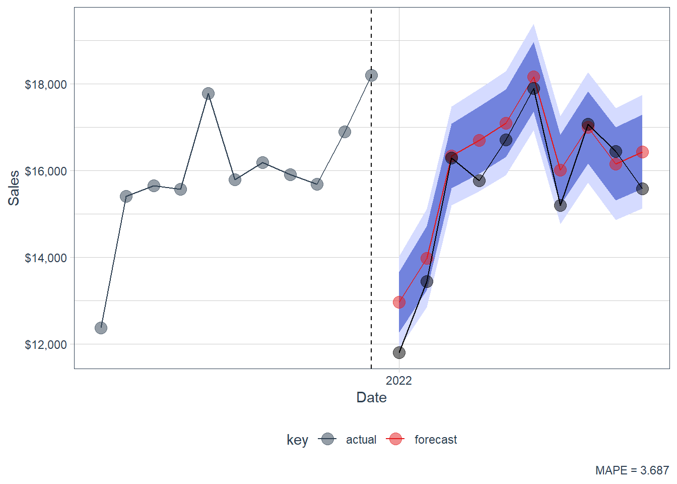
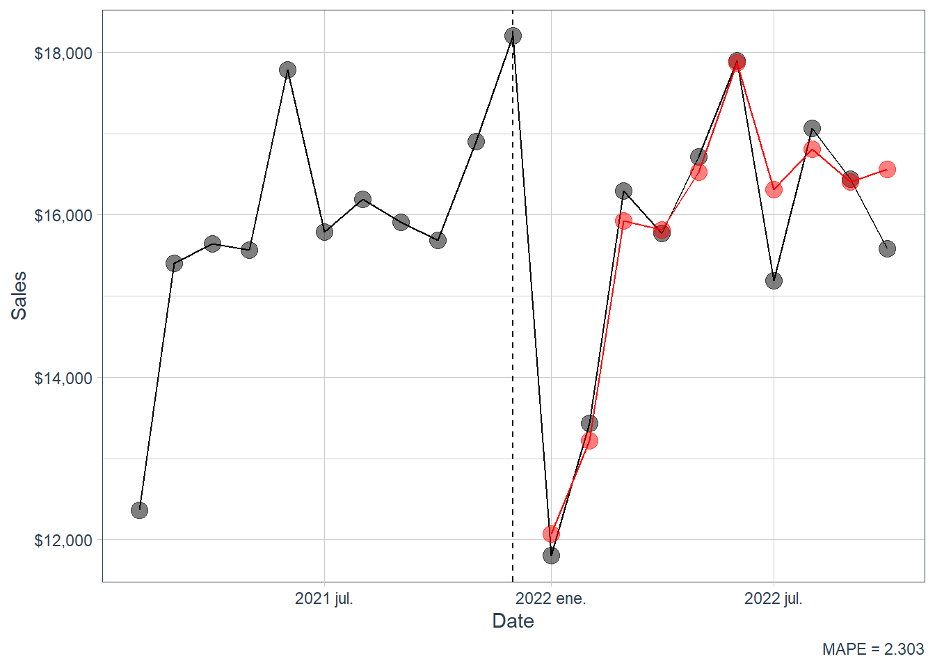
fcast_tbl %>%
  filter(index > as.Date("2021-01-01")) %>%
  ggplot(aes(x = index, y = sales, color = key)) +
  geom_ribbon(aes(ymin = lo.95, ymax = hi.95),
              fill = "#D5DBFF", color = NA, linewidth = 0) +
  geom_ribbon(aes(ymin = lo.80, ymax = hi.80, fill = key),
              fill = "#596DD5", color = NA, linewidth = 0, alpha = 0.8) +
  geom_line() +
  geom_point(size = 4, alpha = 0.5) +
  geom_line(aes(x = date, y = sales), color = "black",
            data = actuals_tbl) +
  geom_point(aes(x = date, y = sales), color = "black", size = 4,
             alpha = 0.5, data = actuals_tbl) +
  geom_vline(xintercept = as.numeric(as.Date("2021-12-01")),
             linetype = 2) +
  labs(x = "Date", y = "Sales",
       caption = paste("MAPE =",
                       round(100 * mean(abs(error_tbl_arima$error_pct)), 5))) +
  scale_x_date(date_breaks = "1 year", date_labels = "%Y") +
  scale_color_tq() +
  scale_fill_tq() +
  theme_tq() +
  scale_y_continuous(labels = scales::dollar)

Figure 2.5: Forecast. forecast::auto.arima.

The resulting forecast serves as a benchmark.

In this render, forecast::auto.arima has MAPE around 3.69. This makes it a strong benchmark: it beats the supervised machine-learning forecasts in this specific holdout period and lands close to the best models from the first chapter. That result is pedagogically useful because it shows that classical time-series structure can remain highly competitive when the series has strong trend, seasonality and autocorrelation.

2.6 Summary of all results

An interesting question is: What happens to the accuracy when you average the predictions of different methods? This question makes sense because model choice is often uncertain in forecasting. Taking the average can reduce extreme results, although it can also be harder to interpret because the final forecast comes from several techniques.

If there are \(M\) forecast models, the average forecast is

\[ \hat{y}^{\text{avg}}_t = \frac{1}{M}\sum_{m=1}^{M}\hat{y}^{(m)}_t. \]

This ensemble rule is applied after the individual forecasts already exist. Its appeal is that different models can make different errors, so averaging may reduce model-specific noise. Its cost is interpretability: the final number no longer comes from one clear structural assumption.

In order to calculate the average forecast we need to load the forecasts from the previous section. In particular, we include the seasonal naive, NNAR(15,1,8)[12], ETS(M,A,M), and ARIMA(4,1,1)(0,1,1)[12]. We exclude the naive, drift and mean forecasts from this average.

fpp3_fc <- readRDS("fpp3_fc.rds")

We add the machine-learning forecasts and the forecast::auto.arima forecast into the fpp3 forecast table.

ml_fc <- ml_errors %>%
  transmute(.model = model, date = yearmonth(date), .mean = pred) %>%
  as_tsibble(key = .model, index = date)

pred_arima_fc <- error_tbl_arima %>%
  transmute(.model = "forecast::auto.arima",
            date = yearmonth(date),
            .mean = pred) %>%
  as_tsibble(key = .model, index = date)

all_fc <- as_tsibble(fpp3_fc) %>%
  select(.model, date, .mean) %>%
  bind_rows(ml_fc, pred_arima_fc)

average <- all_fc %>%
  index_by(date) %>%
  summarise(av_fc = mean(.mean, na.rm = TRUE)) %>%
  bind_cols(sales = actuals_tbl$sales) %>%
  mutate(error = round((sales - av_fc), 2),
         error_pct = round((error / sales), 4))

average

# A tsibble: 10 x 5 [1M]
        date  av_fc sales   error error_pct
       <mth>  <dbl> <int>   <dbl>     <dbl>
 1 2022 ene. 12071. 11801  -270.    -0.0228
 2 2022 feb. 13222. 13435   213.     0.0159
 3 2022 mar. 15926. 16292   366.     0.0224
 4 2022 abr. 15817. 15772   -44.7   -0.0028
 5 2022 may. 16522. 16714   192.     0.0115
 6 2022 jun. 17871. 17899    28.2    0.0016
 7 2022 jul. 16310. 15193 -1117.    -0.0735
 8 2022 ago. 16805. 17069   264.     0.0155
 9 2022 sep. 16409. 16443    33.6    0.002 
10 2022 oct. 16557. 15585  -972.    -0.0623

Finally, the average forecast.

beer %>%
  filter(date > as.Date("2021-01-01")) %>%
  ggplot(aes(x = yearmonth(date), y = sales)) +
  geom_line(color = "black", linewidth = 0.5) +
  geom_point(color = "black", size = 4, alpha = 0.5) +
  geom_line(aes(y = av_fc), linewidth = 0.5,
            color = "red", data = average) +
  geom_point(aes(y = av_fc), size = 4, alpha = 0.5,
             color = "red", data = average) +
  geom_vline(xintercept = as.numeric(as.Date("2021-12-01")), linetype = 2) +
  theme_tq() +
  labs(x = "Date", y = "Sales",
       caption = paste("MAPE =",
                       round(100 * mean(abs(average$error_pct)), 5))) +
  scale_y_continuous(labels = scales::dollar)

Figure 2.6: Forecast. Average.

The final MAPE summary is updated with the ARIMA benchmark and the average forecast.

mape_updated_all <- mape_updated_ml %>%
  add_row(.model = "forecast::auto.arima",
          MAPE = 100 * mean(abs(error_tbl_arima$error_pct))) %>%
  add_row(.model = "Average forecast",
          MAPE = 100 * mean(abs(average$error_pct))) %>%
  arrange(MAPE)

mape_updated_all

# A tibble: 12 × 2
   .model                          MAPE
   <chr>                          <dbl>
 1 Average forecast                2.30
 2 forecast::auto.arima            3.69
 3 fpp3: ETS(M,A,M)                3.77
 4 fpp3: seasonal naïve            3.89
 5 fpp3: ARIMA(4,1,1)(0,1,1)[12]   4.40
 6 ML forecast: neural network     4.91
 7 ML forecast: regression tree    5.16
 8 ML forecast: linear regression  5.81
 9 fpp3: NNAR(15,1,8)[12]          6.02
10 fpp3: naïve                    18.1 
11 fpp3: drift                    20.9 
12 fpp3: mean                     23.5 

The ranking is local to this data set and this holdout period. The main lesson is that a transparent workflow lets us see where the forecast comes from, how the model was selected, how long it takes to render, and how it performs when confronted with truly unseen data.

The average forecast is the best row in this render, with MAPE around 2.37. That result has a clear interpretation: the individual models make different errors, and averaging reduces part of that model-specific noise. The cost is interpretability because the final number comes from several forecasting rules. For teaching purposes, this is a valuable ending point: students can see that the best empirical forecast may come from combining models, while the individual models remain necessary for understanding what information the forecast is using.

2.7 References

The main web references of this document are:

• Time Series Machine Learning with timetk.
• Tidy Forecasting with sweep.
• Forecasting: Principles and Practice.