3 GARCH volatility forecasting in R
3.1 Volatility as a forecasting problem
The previous chapters forecast the level of a monthly sales series. Here the forecast target changes. We work with daily financial returns and forecast conditional variance, the variance expected for the next period using the information available today. The implementation is adapted from the original pedagogical GARCH material in Lozano (2025) and rewritten here as a Quarto book chapter focused on applied forecasting.
In financial time series, large movements tend to cluster. Calm periods can last for many days, and turbulent periods can also persist. A single unconditional standard deviation summarizes the full sample with one number. A GARCH model produces a time series of conditional volatility, which is useful precisely because risk changes through time. This risk-management motivation is standard in financial engineering and quantitative risk management; see Hull (2022) and McNeil et al. (2015).
Let \(u_t\) be the daily return and let \(\mathcal{F}_{t-1}\) denote the information available at the end of day \(t-1\). The object of interest is
\[ v_t = \operatorname{Var}(u_t \mid \mathcal{F}_{t-1}), \]
where \(v_t=\sigma_t^2\) is the conditional variance. The corresponding conditional volatility is \(\sigma_t=\sqrt{v_t}\).
We build the model manually so the bridge remains visible:
\[ \text{returns} \longrightarrow \text{GARCH recursion} \longrightarrow \text{likelihood} \longrightarrow \text{estimated volatility} \longrightarrow \text{volatility forecast}. \]
3.2 Returns and data preparation
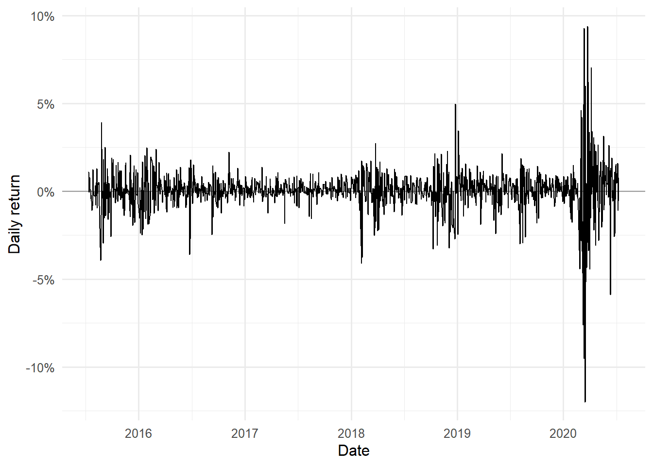
The empirical example uses the S&P 500 index from 2015-07-10 to 2020-07-10. Let \(S_t\) be the closing index level. The simple daily return is
\[ u_t = \frac{S_t-S_{t-1}}{S_{t-1}} = \frac{S_t}{S_{t-1}}-1. \]
Returns are more appropriate than prices for daily volatility analysis because they measure relative changes. The square \(u_t^2\) measures the size of the shock regardless of sign.
Code
sp500 <- tq_get("^GSPC", from = "2015-07-10", to = "2020-07-10") |>
  select(date, close) |>
  rename(price = close) |>
  mutate(
    return = price / lag(price) - 1
  )

sp500 |>
  select(date, price, return) |>
  slice(c(1:6, (n() - 1):n())) |>
  kable(
    caption = "S&P 500 prices and simple daily returns.",
    digits = 8,
    format.args = list(scientific = FALSE),
    row.names = FALSE
  ) |>
kable_styling(latex_options = "HOLD_position")| date | price | return |
|---|---|---|
| 2015-07-10 | 2076.62 | NA |
| 2015-07-13 | 2099.60 | 0.01106605 |
| 2015-07-14 | 2108.95 | 0.00445316 |
| 2015-07-15 | 2107.40 | -0.00073499 |
| 2015-07-16 | 2124.29 | 0.00801468 |
| 2015-07-17 | 2126.64 | 0.00110618 |
| 2020-07-08 | 3169.94 | 0.00782746 |
| 2020-07-09 | 3152.05 | -0.00564361 |
The first return is missing because the first row has no previous closing price. We estimate the model after removing that first missing value.
The following plot shows why a conditional volatility model is useful. Large absolute returns appear in clusters, especially around the 2020 market stress episode.
Code
3.3 The GARCH(1,1) model
The GARCH(1,1) model of Bollerslev (1986) extends the ARCH idea of Engle (1982) by allowing conditional variance to depend on a recent shock and on its own previous value. Broader treatments of financial time series and GARCH modeling are given in Tsay (2010), Ruppert (2011), and Francq and Zakoian (2019).
\[ v_t = \omega + \alpha u_{t-1}^2 + \beta v_{t-1}. \]
The model has three parameters:
| Parameter | Interpretation |
|---|---|
| \(\omega\) | Baseline variance component. |
| \(\alpha\) | Reaction to the most recent squared return. |
| \(\beta\) | Persistence from the previous conditional variance. |
The usual restrictions are
\[ \omega>0, \qquad \alpha \ge 0, \qquad \beta \ge 0, \qquad \alpha+\beta<1. \]
The last restriction gives a finite long-run variance. The sum \(\alpha+\beta\) is especially important: it measures volatility persistence. If the sum is close to one, shocks fade slowly.
The long-run variance implied by a stationary GARCH(1,1) is
\[ \bar{v} = \frac{\omega}{1-\alpha-\beta}. \]
This identity will be used later for variance targeting and for multi-step volatility forecasts.
3.4 Conditional variance recursion
The model is recursive. To compute \(v_t\), the code needs \(u_{t-1}^2\) and \(v_{t-1}\). The first conditional variance must therefore be initialized. To preserve the source example, we use the shifted initialization from the original Hull-style material: the first available squared return initializes the second variance value. The first return is therefore used to start the recursion, and the likelihood is evaluated from the observations with valid conditional variance.
The mapping from notation to R is direct:
| Mathematical object | R object |
|---|---|
| \(u_t\) | u[t] |
| \(v_t\) | v[t] |
| \(\omega\) | omega |
| \(\alpha\) | alpha |
| \(\beta\) | beta |
The body of the loop mirrors the equation. The code uses u[t - 1]^2 for the shock term and v[t - 1] for the lagged conditional variance. The shifted initialization makes the alignment explicit: u[1]^2 initializes v[2], and the recursive GARCH update begins at t = 3.
3.5 Maximum likelihood estimation
After defining the recursion, we need a statistical criterion for estimating the parameters. For this teaching example, returns are assumed to be conditionally normal with zero conditional mean:
\[ u_t \mid \mathcal{F}_{t-1} \sim \mathcal{N}(0,v_t). \]
This assumption gives the log-likelihood contribution
\[ \ell_t^\ast = -\log(v_t) - \frac{u_t^2}{v_t}. \]
This is the proportional log-likelihood used in the source example. It omits constants and multiplies the normal log-likelihood by a positive factor, so the optimizer searches the same parameter region while preserving the original reported scale. Since optim() minimizes, the R function below returns the negative of this criterion. Parameter restrictions are handled inside the function. Invalid parameter vectors receive a very large objective value. For a more formal treatment of GARCH likelihood, stationarity, and inference, see Francq and Zakoian (2019).
The zero-mean assumption keeps the chapter focused on volatility. In a broader empirical application, \(u_t\) could be replaced by residuals from a mean model, such as a constant-mean or ARMA specification.
Because the shifted recursion leaves the first variance value undefined, the likelihood below is conditional on the valid variance values produced by the recursion. The same convention is used for both estimators, so the comparison remains internally consistent.
Code
nll_garch <- function(par, u) {
  omega <- par[1]
  alpha <- par[2]
  beta <- par[3]

  if (omega <= 0 || alpha < 0 || beta < 0 || (alpha + beta) >= 1) {
    return(1e12)
  }

  v <- garch_variance(u, omega, alpha, beta)
  valid <- !is.na(v) & v > 0

  if (!any(valid)) {
    return(1e12)
  }

  -sum(-log(v[valid]) - (u[valid]^2) / v[valid])
}
3.6 Full MLE results
Full maximum likelihood estimates the three GARCH parameters \((\omega,\alpha,\beta)\). We keep the original numerical strategy: L-BFGS-B handles simple lower and upper bounds, and the objective function penalizes parameter vectors that violate \(\alpha+\beta<1\).
Code
start <- c(omega = 4e-6, alpha = 0.2, beta = 0.7)

fit_full <- optim(
  par = start,
  fn = nll_garch,
  u = u,
  method = "L-BFGS-B",
  lower = c(1e-12, 0, 0),
  upper = c(Inf, 1 - 1e-6, 1 - 1e-6)
)

theta_full <- fit_full$par
omega_full <- theta_full["omega"]
alpha_full <- theta_full["alpha"]
beta_full <- theta_full["beta"]

v_full <- garch_variance(u, omega_full, alpha_full, beta_full)
valid_full <- !is.na(v_full) & v_full > 0

loglik_full <- -nll_garch(theta_full, u)
n_full <- sum(valid_full)
k_full <- 3
aic_full <- -2 * loglik_full + 2 * k_full
bic_full <- -2 * loglik_full + log(n_full) * k_full

ab_full <- alpha_full + beta_full
half_life_full <- ifelse(ab_full < 1, log(0.5) / log(ab_full), NA_real_)

full_summary <- tibble(
  metric = c(
    "omega",
    "alpha",
    "beta",
    "alpha + beta",
    "half-life in trading days",
    "logLik",
    "n_obs",
    "AIC",
    "BIC"
  ),
  value = c(
    omega_full,
    alpha_full,
    beta_full,
    ab_full,
    half_life_full,
    loglik_full,
    n_full,
    aic_full,
    bic_full
  )
)

full_summary |>
  kable(
    caption = "Full maximum likelihood GARCH(1,1) estimates.",
    digits = 6,
    row.names = FALSE
  ) |>
kable_styling(latex_options = "HOLD_position")| metric | value |
|---|---|
| omega | 0.000003 |
| alpha | 0.229733 |
| beta | 0.758404 |
| alpha + beta | 0.988138 |
| half-life in trading days | 58.086329 |
| logLik | 10835.375594 |
| n_obs | 1257.000000 |
| AIC | -21664.751188 |
| BIC | -21649.341739 |
The parameter \(\alpha\) measures the immediate response to a new shock. The parameter \(\beta\) measures persistence. Their sum measures how slowly conditional variance returns toward its long-run level. The half-life translates that persistence into trading days:
\[ \text{half-life} = \frac{\log(0.5)}{\log(\alpha+\beta)}. \]
3.7 Variance targeting
Variance targeting changes how \(\omega\) is identified. The method fixes a long-run variance level \(V_L\) and uses the stationary GARCH identity
\[ \omega = V_L(1-\alpha-\beta). \]
In this chapter, \(V_L\) is the sample variance of returns. The estimation problem then has two free parameters, \((\alpha,\beta)\), and \(\omega\) is calculated from the long-run variance condition.
Code
nll_garch_vt <- function(par, u, long_run_variance) {
  alpha <- par[1]
  beta <- par[2]

  if (alpha < 0 || beta < 0 || (alpha + beta) >= 1) {
    return(1e12)
  }

  omega <- long_run_variance * (1 - alpha - beta)
  v <- garch_variance(u, omega, alpha, beta)
  valid <- !is.na(v) & v > 0

  if (!any(valid)) {
    return(1e12)
  }

  -sum(-log(v[valid]) - (u[valid]^2) / v[valid])
}

fit_vt <- optim(
  par = c(alpha = 0.2, beta = 0.7),
  fn = nll_garch_vt,
  u = u,
  long_run_variance = long_run_variance,
  method = "L-BFGS-B",
  lower = c(0, 0),
  upper = c(1 - 1e-6, 1 - 1e-6)
)

alpha_vt <- fit_vt$par["alpha"]
beta_vt <- fit_vt$par["beta"]
omega_vt <- long_run_variance * (1 - alpha_vt - beta_vt)

v_vt <- garch_variance(u, omega_vt, alpha_vt, beta_vt)
valid_vt <- !is.na(v_vt) & v_vt > 0

loglik_vt <- -nll_garch_vt(fit_vt$par, u, long_run_variance)
n_vt <- sum(valid_vt)
k_vt <- 2
aic_vt <- -2 * loglik_vt + 2 * k_vt
bic_vt <- -2 * loglik_vt + log(n_vt) * k_vt

ab_vt <- alpha_vt + beta_vt
half_life_vt <- ifelse(ab_vt < 1, log(0.5) / log(ab_vt), NA_real_)

vt_summary <- tibble(
  metric = c(
    "omega",
    "alpha",
    "beta",
    "alpha + beta",
    "half-life in trading days",
    "logLik",
    "n_obs",
    "AIC",
    "BIC"
  ),
  value = c(
    omega_vt,
    alpha_vt,
    beta_vt,
    ab_vt,
    half_life_vt,
    loglik_vt,
    n_vt,
    aic_vt,
    bic_vt
  )
)

vt_summary |>
  kable(
    caption = "Variance targeting GARCH(1,1) estimates.",
    digits = 6,
    row.names = FALSE
  ) |>
kable_styling(latex_options = "HOLD_position")| metric | value |
|---|---|
| omega | 0.000004 |
| alpha | 0.226349 |
| beta | 0.747038 |
| alpha + beta | 0.973387 |
| half-life in trading days | 25.696953 |
| logLik | 10837.404644 |
| n_obs | 1257.000000 |
| AIC | -21670.809288 |
| BIC | -21660.536321 |
Variance targeting is a modeling restriction. It reduces the number of optimized parameters and anchors the long-run variance level. That can improve numerical stability and communication, provided that the chosen long-run variance is appropriate for the sample.
3.8 Objective surface and estimator comparison
Variance targeting leaves only two optimized parameters, so the objective function can be visualized on the \((\alpha,\beta)\) plane. This plot connects the code to the estimation logic: optim() searches over pairs \((\alpha,\beta)\), evaluates the criterion, and returns the pair with the lowest objective value. The contour labels use the equivalent proportional log-likelihood scale, where larger values correspond to lower objective values. The axis limits keep the same window as the source example, so the solution remains visible in the relevant region.
Code
alpha_grid <- seq(0.22, 0.30, length.out = 100)
beta_grid <- seq(0.66, 0.76, length.out = 100)

objective_surface <- outer(alpha_grid, beta_grid, Vectorize(function(alpha, beta) {
  if (alpha < 0 || beta < 0 || (alpha + beta) >= 0.999) {
    return(NA_real_)
  }

  nll_garch_vt(c(alpha, beta), u = u, long_run_variance = long_run_variance)
}))

loglik_surface <- -objective_surface
contour_levels <- c(10700, 10750, 10800, 10820, 10830, 10835)

contour_lines <- grDevices::contourLines(
  x = beta_grid,
  y = alpha_grid,
  z = t(loglik_surface),
  levels = contour_levels
)

contour_tbl <- bind_rows(lapply(seq_along(contour_lines), function(id) {
  tibble(
    contour_id = id,
    beta = contour_lines[[id]]$x,
    alpha = contour_lines[[id]]$y,
    log_likelihood = contour_lines[[id]]$level
  )
}))

label_candidates <- contour_tbl |>
  filter(
    beta >= 0.662,
    beta <= 0.756,
    alpha >= 0.225,
    alpha <= 0.285
  )

level_tbl <- tibble(
  log_likelihood = contour_levels,
  label_beta_target = c(0.715, 0.730, 0.743, 0.748, 0.752, 0.755)
)

contour_label_tbl <- label_candidates |>
  inner_join(level_tbl, by = "log_likelihood") |>
  group_by(log_likelihood) |>
  slice_min(abs(beta - label_beta_target), n = 1, with_ties = FALSE) |>
  ungroup() |>
  mutate(label = scales::number(log_likelihood, accuracy = 1, big.mark = ""))

solution_tbl <- tibble(
  beta = beta_vt,
  alpha = alpha_vt
)

contour_tbl |>
  ggplot(aes(beta, alpha)) +
  geom_path(aes(group = contour_id), color = "#1B4E8A", linewidth = 0.5) +
  geom_label(
    data = contour_label_tbl,
    aes(label = label),
    color = "#2F2F2F",
    fill = "white",
    label.size = 0,
    size = 3,
    alpha = 0.9
  ) +
  geom_hline(yintercept = alpha_vt, color = "#B22222", linetype = 2) +
  geom_vline(xintercept = beta_vt, color = "#B22222", linetype = 2) +
  geom_point(
    data = solution_tbl,
    color = "#B22222",
    size = 2.8
  ) +
  coord_cartesian(xlim = c(0.66, 0.76), ylim = c(0.22, 0.30), expand = FALSE) +
  labs(
    x = expression(beta),
    y = expression(alpha),
    caption = "Contour labels show proportional log-likelihood values; higher values imply a lower objective."
  ) +
  theme_minimal(base_size = 12) +
  theme(legend.position = "none")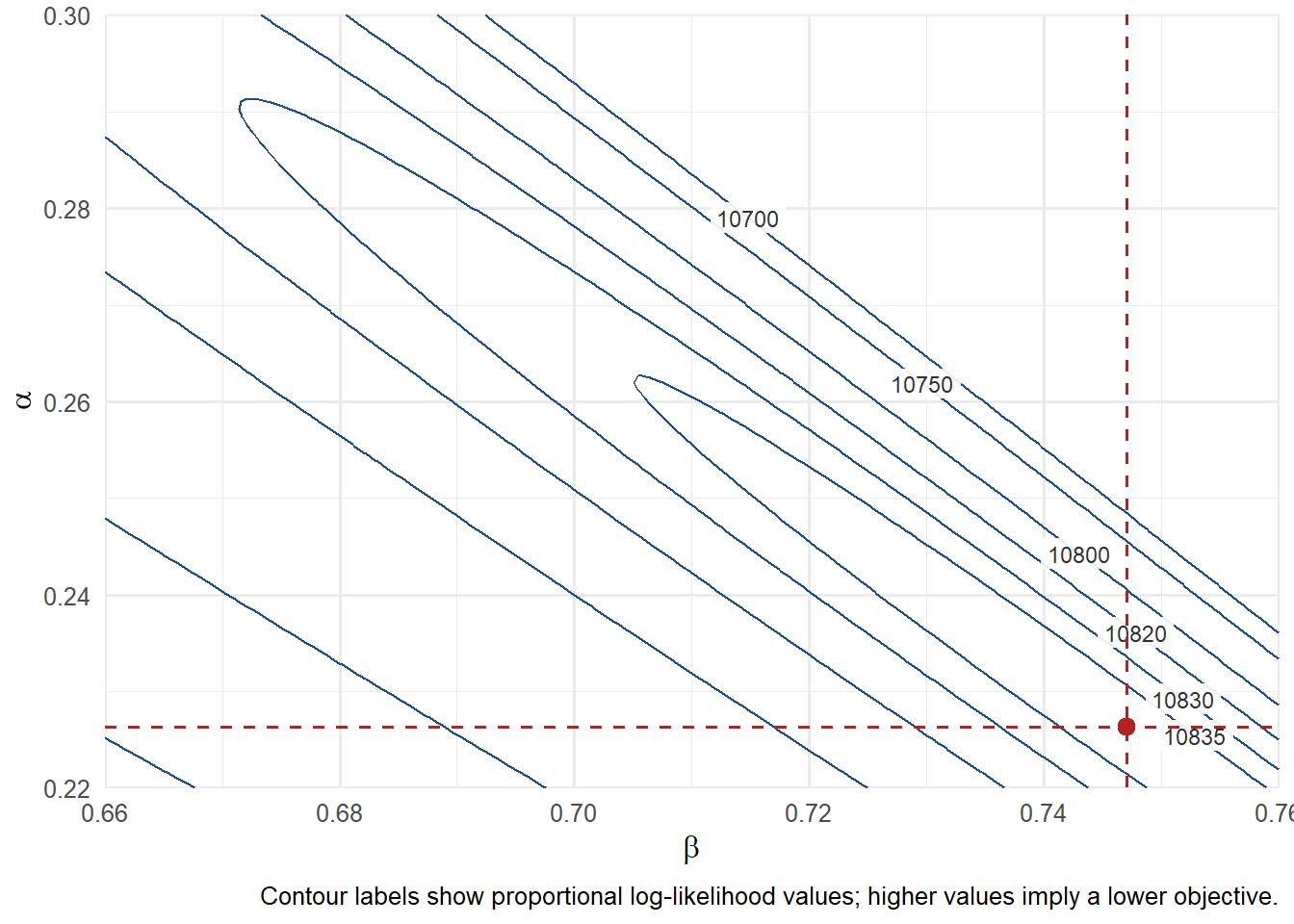
The red point marks the solution returned by optim(). The labels on the contours make the surface easier to read: moving toward higher log-likelihood values moves toward the criterion that optim() minimizes. Long and flat contours would suggest that several combinations of \(\alpha\) and \(\beta\) produce similar criterion values.
The two estimators use the same GARCH recursion. The difference is how much structure they impose on \(\omega\).
Code
comparison_tbl <- bind_rows(
  full_summary |> mutate(model = "Full MLE"),
  vt_summary |> mutate(model = "Variance targeting")
) |>
  pivot_wider(names_from = model, values_from = value) |>
  select(metric, `Full MLE`, `Variance targeting`)

comparison_tbl |>
  kable(
    caption = "Full MLE and variance targeting comparison.",
    digits = 6,
    row.names = FALSE
  ) |>
kable_styling(latex_options = "HOLD_position")| metric | Full MLE | Variance targeting |
|---|---|---|
| omega | 0.000003 | 0.000004 |
| alpha | 0.229733 | 0.226349 |
| beta | 0.758404 | 0.747038 |
| alpha + beta | 0.988138 | 0.973387 |
| half-life in trading days | 58.086329 | 25.696953 |
| logLik | 10835.375594 | 10837.404644 |
| n_obs | 1257.000000 | 1257.000000 |
| AIC | -21664.751188 | -21670.809288 |
| BIC | -21649.341739 | -21660.536321 |
The log-likelihood column uses the same proportional criterion as the source example. AIC and BIC are therefore read on the scale of that convention. They add a penalty for the number of estimated parameters: Full MLE uses three parameters, while variance targeting optimizes two parameters and treats \(V_L\) as a fixed plug-in anchor. With that convention, the comparison is about fit and parsimony together. This style of comparison is common in applied financial time-series work, where likelihood fit, parameter plausibility, and residual diagnostics are read together (Tsay 2010; Ruppert 2011).
The main economic reading comes from \(\alpha\), \(\beta\), and \(\alpha+\beta\). Similar values across the two estimators indicate that the long-run variance restriction does not radically change the shock reaction and persistence estimates in this sample. The larger difference is in \(\alpha+\beta\): Full MLE is closer to the persistence boundary, while variance targeting gives a shorter half-life. That comparison helps students see that both estimators share the same recursion, yet the restriction on \(\omega\) changes how persistence and long-run variance are balanced.
3.9 Conditional volatility through time and forecasts
The most useful output is the conditional volatility series. We use the variance targeting estimates for the plot because they are parsimonious and produce the long-run level explicitly. The same reconstruction can be done with the Full MLE estimates. Conditional volatility links this chapter to risk measurement, scenario analysis, and derivatives applications (Hull 2022; McNeil et al. 2015).
Code
volatility_tbl <- returns |>
  mutate(
    variance_vt = v_vt,
    volatility_vt = sqrt(variance_vt),
    sample_volatility = sqrt(long_run_variance)
  )

volatility_tbl |>
  select(date, return, variance_vt, volatility_vt) |>
  slice(c(1:6, (n() - 1):n())) |>
  kable(
    caption = "Conditional variance and volatility from variance targeting.",
    digits = 8,
    format.args = list(scientific = FALSE),
    row.names = FALSE
  ) |>
kable_styling(latex_options = "HOLD_position")| date | return | variance_vt | volatility_vt |
|---|---|---|---|
| 2015-07-13 | 0.01106605 | NA | NA |
| 2015-07-14 | 0.00445316 | 0.00012246 | 0.01106605 |
| 2015-07-15 | -0.00073499 | 0.00009994 | 0.00999677 |
| 2015-07-16 | 0.00801468 | 0.00007874 | 0.00887379 |
| 2015-07-17 | 0.00110618 | 0.00007733 | 0.00879379 |
| 2015-07-20 | 0.00077123 | 0.00006201 | 0.00787479 |
| 2020-07-08 | 0.00782746 | 0.00016849 | 0.01298025 |
| 2020-07-09 | -0.00564361 | 0.00014370 | 0.01198752 |
Code
volatility_tbl |>
  ggplot(aes(date, 100 * volatility_vt)) +
  geom_line(color = "#1B4E8A", linewidth = 0.6) +
  geom_hline(
    aes(yintercept = 100 * sample_volatility),
    color = "#B22222",
    linetype = 2
  ) +
  labs(
    x = "Date",
    y = "Daily volatility",
    caption = "Dashed line: sample daily volatility."
  ) +
  scale_y_continuous(labels = scales::label_percent(accuracy = 0.1, scale = 1)) +
  theme_minimal(base_size = 12)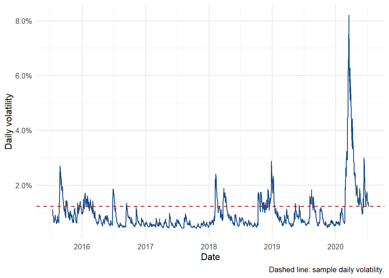
The model assigns more volatility to turbulent periods and less volatility to calm periods. That is the practical contribution of GARCH relative to a single sample standard deviation.
After reconstructing the historical conditional volatility path, the final step is an explicit volatility forecast. Let \(T\) be the last observed day. The one-step-ahead forecast is
\[ \hat{v}_{T+1\mid T} = \omega + \alpha u_T^2 + \beta v_T. \]
For horizons beyond one day, the expected future squared shock is the future conditional variance. The GARCH(1,1) forecast therefore reverts toward the long-run variance:
\[ \hat{v}_{T+h\mid T} = \bar{v} + (\alpha+\beta)^{h-1} \left( \hat{v}_{T+1\mid T}-\bar{v} \right), \qquad h \ge 1. \]
Code
last_return <- tail(u, 1)
last_variance <- tail(v_vt, 1)

v_next <- omega_vt + alpha_vt * last_return^2 + beta_vt * last_variance
long_run_vt <- omega_vt / (1 - alpha_vt - beta_vt)

horizon <- 20
forecast_variance <- long_run_vt +
  (alpha_vt + beta_vt)^(seq_len(horizon) - 1) * (v_next - long_run_vt)

forecast_tbl <- tibble(
  horizon = seq_len(horizon),
  variance_forecast = forecast_variance,
  volatility_forecast = sqrt(forecast_variance)
)

forecast_tbl |>
  kable(
    caption = "Twenty-day conditional volatility forecast.",
    digits = 8,
    format.args = list(scientific = FALSE),
    row.names = FALSE
  ) |>
kable_styling(latex_options = "HOLD_position")| horizon | variance_forecast | volatility_forecast |
|---|---|---|
| 1 | 0.00011853 | 0.01088694 |
| 2 | 0.00011934 | 0.01092416 |
| 3 | 0.00012013 | 0.01096028 |
| 4 | 0.00012090 | 0.01099532 |
| 5 | 0.00012165 | 0.01102932 |
| 6 | 0.00012237 | 0.01106232 |
| 7 | 0.00012308 | 0.01109435 |
| 8 | 0.00012378 | 0.01112543 |
| 9 | 0.00012445 | 0.01115560 |
| 10 | 0.00012510 | 0.01118489 |
| 11 | 0.00012574 | 0.01121333 |
| 12 | 0.00012636 | 0.01124095 |
| 13 | 0.00012696 | 0.01126776 |
| 14 | 0.00012755 | 0.01129380 |
| 15 | 0.00012812 | 0.01131909 |
| 16 | 0.00012868 | 0.01134365 |
| 17 | 0.00012922 | 0.01136750 |
| 18 | 0.00012975 | 0.01139068 |
| 19 | 0.00013026 | 0.01141319 |
| 20 | 0.00013076 | 0.01143506 |
Code
forecast_tbl |>
  ggplot(aes(horizon, 100 * volatility_forecast)) +
  geom_line(color = "#1B4E8A", linewidth = 0.8) +
  geom_point(color = "#1B4E8A", size = 2) +
  geom_hline(
    yintercept = 100 * sqrt(long_run_vt),
    color = "#B22222",
    linetype = 2
  ) +
  labs(
    x = "Forecast horizon in trading days",
    y = "Daily volatility forecast",
    caption = "Dashed line: variance targeting long-run volatility."
  ) +
  scale_y_continuous(labels = scales::label_percent(accuracy = 0.1, scale = 1)) +
  theme_minimal(base_size = 12)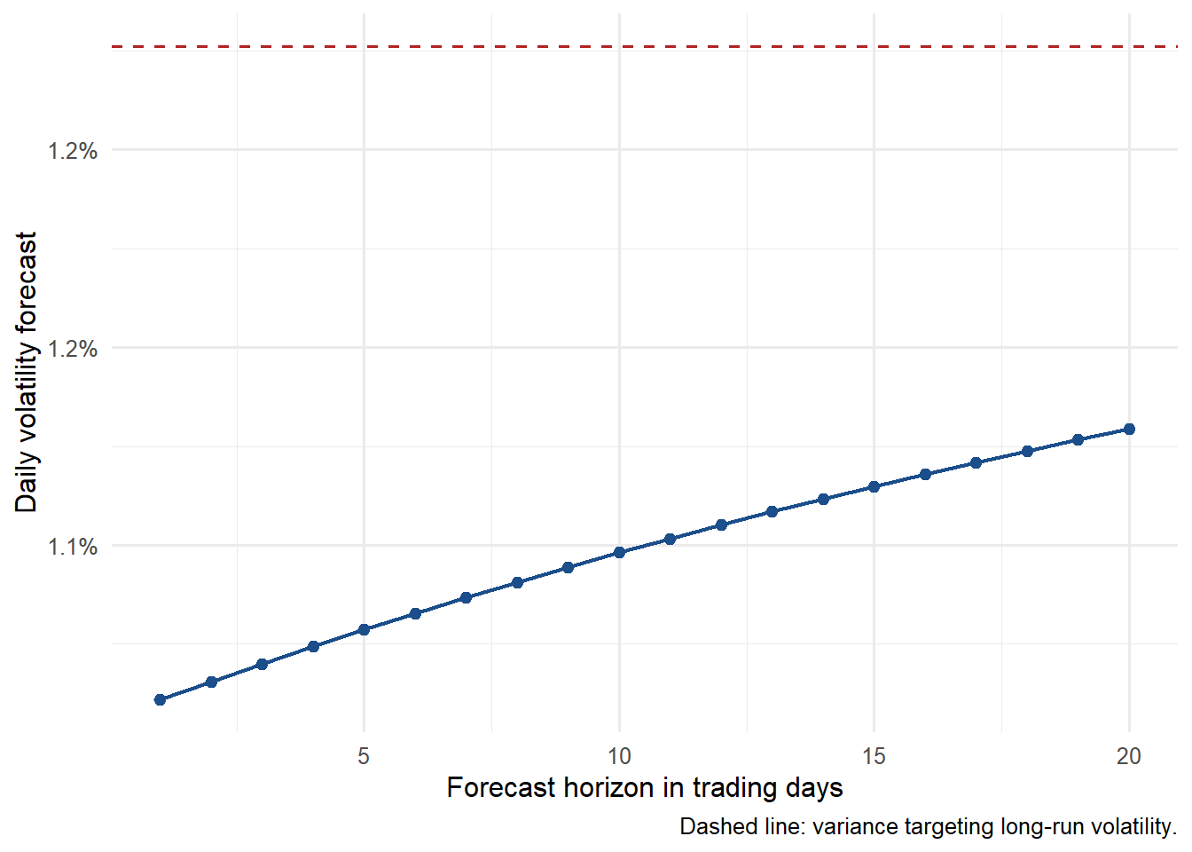
This is a risk forecast. Its target is the expected size of future return variation under the estimated GARCH dynamics; directional return forecasting is outside this chapter’s target.
3.10 Residual diagnostics
After estimating a volatility model, we check whether the standardized residuals look closer to white noise. The standardized residual is
\[ z_t = \frac{u_t}{\sqrt{\hat{v}_t}}. \]
If GARCH captures the main volatility clustering, the squared standardized residuals should have less autocorrelation than the squared raw returns.
Code
diag_tbl <- volatility_tbl |>
  filter(!is.na(variance_vt), variance_vt > 0) |>
  mutate(
    z = return / sqrt(variance_vt),
    z_squared = z^2
  )

lb_z <- stats::Box.test(diag_tbl$z, lag = 20, type = "Ljung-Box")
lb_z_squared <- stats::Box.test(diag_tbl$z_squared, lag = 20, type = "Ljung-Box")

diag_tests <- tibble(
  test = c("Ljung-Box on z_t", "Ljung-Box on z_t squared"),
  statistic = c(as.numeric(lb_z$statistic), as.numeric(lb_z_squared$statistic)),
  p_value = c(lb_z$p.value, lb_z_squared$p.value)
)

diag_tests |>
  kable(
    caption = "Residual diagnostic tests.",
    digits = 4,
    row.names = FALSE
  ) |>
kable_styling(latex_options = "HOLD_position")| test | statistic | p_value |
|---|---|---|
| Ljung-Box on z_t | 12.9968 | 0.8775 |
| Ljung-Box on z_t squared | 14.0188 | 0.8295 |
Code
acf_squared <- stats::acf(
  diag_tbl$z_squared,
  plot = FALSE,
  lag.max = 20,
  na.action = na.pass
)

acf_tbl <- tibble(
  lag = as.numeric(acf_squared$lag[-1]),
  acf = as.numeric(acf_squared$acf[-1])
)

acf_tbl |>
  ggplot(aes(lag, acf)) +
  geom_col(width = 0.08, fill = "#1B4E8A") +
  geom_hline(
    yintercept = c(-1.96 / sqrt(nrow(diag_tbl)), 1.96 / sqrt(nrow(diag_tbl))),
    linetype = 2,
    color = "#B22222"
  ) +
  labs(x = "Lag", y = "ACF") +
  theme_minimal(base_size = 12)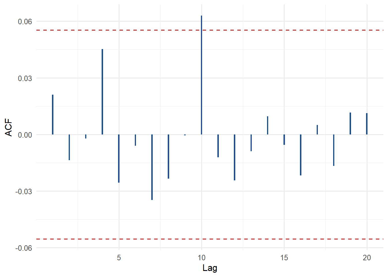
The diagnostic is a model audit. A small p-value for the squared standardized residuals would suggest remaining volatility structure. An ACF with smaller remaining spikes supports the interpretation that the GARCH recursion absorbed much of the conditional heteroskedasticity.
3.11 Common implementation mistakes
A manual GARCH implementation is useful because it makes mistakes visible. The most important checks are:
| Check | Why it is important |
|---|---|
| Lag alignment | The recursion must use \(u_{t-1}^2\) and \(v_{t-1}\) to compute \(v_t\). |
| Scale consistency | Returns should stay in decimal units during estimation. Percent units can be used for plots. |
| Parameter restrictions | \(\omega>0\), \(\alpha\ge0\), \(\beta\ge0\), and \(\alpha+\beta<1\) keep the model interpretable. |
| Starting values | Different feasible starting values should lead to similar estimates in a stable problem. |
| Diagnostics | AIC and BIC should be read together with parameter plausibility and residual checks. |
These checks are part of the model workflow. They protect the correspondence between the equation, the code, and the reported result.
3.12 Conclusion and extensions
This chapter built a GARCH(1,1) volatility forecasting workflow from first principles. The data are daily S&P 500 returns. The model updates conditional variance with the most recent squared return and the previous conditional variance. The likelihood turns that recursion into an estimable criterion, and the estimated parameters produce a conditional volatility series.
Full MLE and variance targeting use the same recursion. Full MLE estimates \((\omega,\alpha,\beta)\) freely. Variance targeting estimates \((\alpha,\beta)\) and constructs \(\omega\) from a long-run variance condition. The comparison therefore teaches a broader modeling lesson: estimation is also a choice about which restrictions are reasonable for the question.
The volatility forecast is the central forecasting object in this chapter. It summarizes expected future risk; directional return forecasting is outside the model target. In an applied forecasting book, that distinction is important: forecasting can target a level, a mean, a probability, or a variance. Here the target is dynamic risk.
The natural extensions follow from the assumptions made here. GARCH(1,1) is a starting point. Common extensions include asymmetric volatility models such as EGARCH and GJR-GARCH, heavy-tailed conditional distributions such as Student-t innovations, and multivariate models such as DCC-GARCH. These extensions are treated in more advanced references such as Francq and Zakoian (2019), Tsay (2010), and McNeil et al. (2015). The core logic remains the same: define a conditional variance process, estimate it with an explicit criterion, diagnose the residuals, and evaluate whether the forecast target is useful for the applied problem.