This chapter studies asset pricing as an applied econometric problem. The goal is to connect factor-model logic, mathematical notation, R code, and empirical interpretation in one continuous workflow. The chapter starts with the economic question, builds the data and test assets, estimates time-series regressions, uses cross-sectional regressions to price factor exposures, and then rewrites the same pricing problem with stochastic discount factor GMM. The emphasis is on making each equation operational: what it means, why it is estimated, how it appears in the code, and how its results should be read.
4.1 Asset pricing as an econometric problem
Asset pricing econometrics asks a precise empirical question: can a small set of systematic risk factors explain why some assets or portfolios earn higher average excess returns than others? The answer is estimated from data, but the data work has to stay connected to the economic model. A coefficient is useful only when the reader can say what it measures, how the code estimated it, and what its value implies for the model.
This chapter follows the regression-based logic used in empirical asset pricing (Cochrane 2005). The same idea appears in three connected forms. Time-series regressions estimate each asset’s exposure to common factors. Cross-sectional regressions ask whether those exposures explain average excess returns across test assets. Stochastic discount factor moments express the same restriction as a pricing condition: after discounting by the model, excess returns should have zero remaining average payoff.
The empirical examples use one mutual fund and the 25 Fama-French size-value portfolios as test assets. The risk factors are the market excess return, size, value, momentum, profitability, and investment factors from the Kenneth French Data Library. The chapter downloads the data during execution and fixes the sample end at 2020-12-31 so the empirical window is reproducible.
The central object is an excess return:
\[
R_{i,t}^e
=
R_{i,t}-R_{f,t},
\]
where \(R_{i,t}\) is the return on asset \(i\) in month \(t\) and \(R_{f,t}\) is the risk-free return. A factor model explains \(R_{i,t}^e\) using common sources of variation. The CAPM uses one factor, the market excess return (Sharpe 1964; Lintner 1965; Mossin 1966). The Fama-French three-factor model adds size and value factors (Fama and French 1992, 1993). Momentum and the five-factor model extend the factor set (Carhart 1997; Fama and French 2015).
The chapter should be read as a sequence of empirical questions. The data tables verify samples, dates, and units. The factor figures show what the explanatory portfolios look like before they become regressors. The time-series regressions translate co-movement into alphas and betas. The cross-sectional regressions then ask whether those estimated exposures, or equivalent return-factor moments, explain average excess returns across the 25 portfolios. The final diagnostic reads the remaining pricing errors by size and value characteristics. Each table and figure therefore has a specific role: audit the data, describe the factors, estimate exposures, diagnose the first pass, test the asset-pricing restriction, or interpret what the model leaves unexplained.
The main vocabulary is:
Concept
Symbol
Reading in the chapter
Test asset
\(i\)
An asset or portfolio whose average excess return the model tries to explain.
Excess return
\(R_{i,t}^e\)
The asset return after subtracting the risk-free rate.
Factor
\(f_{j,t}\)
A common return series used to represent a source of systematic risk.
Beta
\(\beta_{i,j}\)
The exposure of asset \(i\) to factor \(j\), estimated from a time-series regression.
Alpha
\(\alpha_i\)
The average excess return left over after the factor exposures are used.
Price of risk
\(\lambda_j\)
The cross-sectional reward attached to one unit of exposure to factor \(j\).
Pricing error
\(\eta_i\) or \(\alpha_i\)
The part of average return that the model leaves unexplained in the relevant test.
Stochastic discount factor
\(m_t\)
A random discount factor that prices excess returns through moment restrictions.
The chapter uses these concepts in a fixed order. First define excess returns. Then estimate betas and alphas from time-series regressions. Then estimate prices of risk from a cross-section of average returns. Finally inspect pricing errors to see where the model still struggles.
This ordering is useful because asset pricing notation can compress several ideas into one equation. The economic question, the statistical object, and the code object should be separated before they are joined again:
Question
Mathematical object
Code object
Interpretation
What is being explained?
\(\bar{R}_i^e\)
ERe_percent
Average excess return of each test asset.
What is the proposed source of explanation?
\(\mathbf{f}_t\)
Mkt_RF, SMB3, HML, Mom, RMW, CMA
Common factor returns.
How exposed is each asset?
\(\boldsymbol{\beta}_i\)
Time-series lm() coefficients
Sensitivity of asset returns to factor returns.
What does the model leave behind?
\(\alpha_i\) or \(\eta_i\)
Intercepts and fitted-value gaps
Pricing errors.
How is risk priced across assets?
\(\boldsymbol{\lambda}\)
Cross-sectional lm() coefficients
Reward attached to factor exposure.
How does the SDF view express the same restriction?
\(E(m_tR_{i,t}^e)=0\)
Return-factor moments
Discounted excess returns should average to zero.
The word “pricing” should also be read carefully. In this chapter, pricing means testing whether a model can explain average excess returns. For an excess return, the initial cost is zero because the investment is financed at the risk-free rate. A correct model should assign zero value to that excess-return payoff after applying the relevant risk adjustment. That is why alphas, fitted-value gaps, and SDF moments all become ways of measuring pricing errors.
4.2 Data, downloads, and sample construction
The factor data and the 25 size-value portfolio returns are downloaded from the Kenneth French Data Library (French 2026). The individual test asset example uses the Fidelity Contrafund ticker FCNTX downloaded with tidyquant. All returns are converted from percentages to decimal units during estimation. Percent units are used only when a table or graph is meant for interpretation.
The code keeps the data in decimal form. For example, a monthly return of 0.01 means one percent. This convention prevents unit mistakes when returns are added, multiplied, or used in regressions.
The first data audit shows the opening and closing observations of the main data objects. These checks verify dates, decimal units, and column names before any model is estimated.
Code
factor_windows |>mutate(across(c(start, end), as.character)) |>kable(caption ="Sample windows of the downloaded Fama-French data files.",row.names =FALSE ) |>kable_styling(latex_options ="HOLD_position")
Sample windows of the downloaded Fama-French data files.
source
start
end
months
Fama-French 3 factors
1926-07-31
2020-12-31
1134
Momentum factor
1927-01-31
2020-12-31
1128
Fama-French 5 factors
1963-07-31
2020-12-31
690
25 size-value portfolios
1926-07-31
2020-12-31
1134
Code
first_last_rows(ff3_momentum) |>select(date, Mkt_RF, SMB3, HML, Mom, RF) |>kable(caption ="First and last observations of the joined FF3 and momentum sample.",digits =6,row.names =FALSE ) |>kable_styling(latex_options ="HOLD_position")
First and last observations of the joined FF3 and momentum sample.
date
Mkt_RF
SMB3
HML
Mom
RF
1927-01-31
-0.0005
-0.0032
0.0458
0.0057
0.0025
1927-02-28
0.0417
0.0007
0.0272
-0.0150
0.0026
1927-03-31
0.0014
-0.0177
-0.0238
0.0352
0.0030
2020-10-31
-0.0208
0.0434
0.0425
-0.0314
0.0001
2020-11-30
0.1245
0.0581
0.0209
-0.1255
0.0001
2020-12-31
0.0463
0.0501
-0.0168
-0.0237
0.0001
Code
first_last_rows(ff5) |>kable(caption ="First and last observations of the Fama-French five-factor data.",digits =6,row.names =FALSE ) |>kable_styling(latex_options ="HOLD_position")
First and last observations of the Fama-French five-factor data.
date
Mkt_RF
SMB
HML
RMW
CMA
RF
1963-07-31
-0.0039
-0.0048
-0.0081
0.0064
-0.0115
0.0027
1963-08-31
0.0508
-0.0080
0.0170
0.0040
-0.0038
0.0025
1963-09-30
-0.0157
-0.0043
0.0000
-0.0078
0.0015
0.0027
2020-10-31
-0.0208
0.0467
0.0425
-0.0077
-0.0057
0.0001
2020-11-30
0.1244
0.0712
0.0209
-0.0225
0.0128
0.0001
2020-12-31
0.0463
0.0493
-0.0168
-0.0197
-0.0006
0.0001
Code
first_last_rows(portfolios_25) |>select(date, `SMALL LoBM`, `SMALL HiBM`, `BIG LoBM`, `BIG HiBM`) |>kable(caption ="First and last observations of selected 25-portfolio corner returns.",digits =6,row.names =FALSE ) |>kable_styling(latex_options ="HOLD_position")
First and last observations of selected 25-portfolio corner returns.
date
SMALL LoBM
SMALL HiBM
BIG LoBM
BIG HiBM
1926-07-31
0.058276
0.019583
0.033248
0.005623
1926-08-31
-0.020206
0.085104
0.010169
0.077576
1926-09-30
-0.048291
0.008586
-0.012951
-0.024284
2020-10-31
-0.026753
0.012595
-0.045743
0.009898
2020-11-30
0.257600
0.245286
0.107281
0.219976
2020-12-31
0.125156
0.074510
0.053002
0.080558
These tables are a data audit. The window table shows which raw files can be used over which dates. The joined FF3-momentum table then shows the actual intersection used when the model includes momentum, so every displayed column has an observed value for the same month. The first and last rows also confirm that the factor files and the portfolio file are monthly series, expressed in decimal units, and aligned on month-end dates. The selected corner portfolios already hint at the empirical structure used later: small growth, small value, big growth, and big value are the extreme cells of the size-value grid.
4.3 Excess returns and factor notation
The notation in this chapter has three indices in the background. The subscript \(i\) identifies the asset or portfolio. The subscript \(t\) identifies the month. The subscript attached to a beta, such as \(M\), \(S\), or \(H\), identifies the factor. For example, \(\beta_{i,H}\) is the value-factor exposure of asset \(i\), estimated from monthly observations over time.
Each model has an observed left-hand side and estimated right-hand-side coefficients. The observed variable is always an excess return, \(R_{i,t}^e\). The factors are also observed return series. The unknown objects are the intercept and the betas. The regression estimates those unknowns by choosing the line, or plane, that best summarizes the historical relation between the asset’s excess return and the factor returns.
The CAPM time-series regression for asset \(i\) is
where \(MKT_t\) is the market excess return. The intercept \(\alpha_i\) is the average excess return that remains after controlling for market exposure. In a well-specified asset pricing model, alphas should be economically small.
The CAPM is therefore a one-factor claim. It says that market exposure is the relevant systematic risk for expected returns. The regression version asks how strongly each asset moves with the market. The asset-pricing version asks whether that market exposure is enough to account for the asset’s average excess return.
Value factor: high book-to-market minus low book-to-market.
\(MOM_t\)
Momentum factor: recent winners minus recent losers.
\(RMW_t\)
Profitability factor: robust minus weak profitability.
\(CMA_t\)
Investment factor: conservative minus aggressive investment.
Each factor is constructed as a portfolio return. This point is central for the interpretation of betas. A positive loading on \(SMB_t\) means that the asset tends to behave like the small-minus-big portfolio. A positive loading on \(HML_t\) means that the asset tends to behave like the high-book-to-market minus low-book-to-market portfolio. The factor return series already encode the small and value portfolio strategies used in the regression.
The five-factor model replaces the three-factor specification with
The code names these variables as Mkt_RF, SMB3, HML, Mom, SMB5, RMW, and CMA. The distinction between SMB3 and SMB5 is intentional: the size factor in the three-factor data and the size factor in the five-factor data are constructed from different portfolio sorts.
The notation and the code follow the same structure. In the equation, \(R_{i,t}^e\) is the dependent variable and the factors are regressors. In R, Re is the dependent variable and the factor columns appear on the right side of the formula. For example, Re ~ Mkt_RF + SMB3 + HML is the code version of the Fama-French three-factor regression.
4.4 Factor portfolios through time
Before estimating asset pricing regressions, it is useful to inspect the factor returns themselves. The next calculation computes annualized return, annualized volatility, and a simple return-to-risk ratio.
This descriptive step has a practical purpose. A factor is a return series, so it can be read like a portfolio before it is used as a regressor. The annualized table summarizes reward and risk. The cumulative plots show the path by which those rewards are earned over time. The density plots show the distribution of monthly outcomes. The risk-return plots then compress those summaries into a single visual comparison. Together, these checks tell the reader what economic objects enter the regressions.
Annualized performance of the three Fama-French factors and momentum.
factor
months
annualized_return
annualized_volatility
return_per_unit_risk
SMB3
1128
0.0189
0.1097
0.1719
HML
1128
0.0330
0.1220
0.2708
Mkt_RF
1128
0.0662
0.1858
0.3561
Mom
1128
0.0621
0.1638
0.3794
The annualized table turns each factor into an object that can be compared like a portfolio. The return column shows the long-run reward, the volatility column shows the risk of the factor strategy, and the return-per-risk column gives a compact scale for ranking factor performance before looking at individual assets.
The three-factor file is inspected first by itself. This mirrors the original workflow: read the Fama-French factors, check their time path, and then add momentum as an extension.
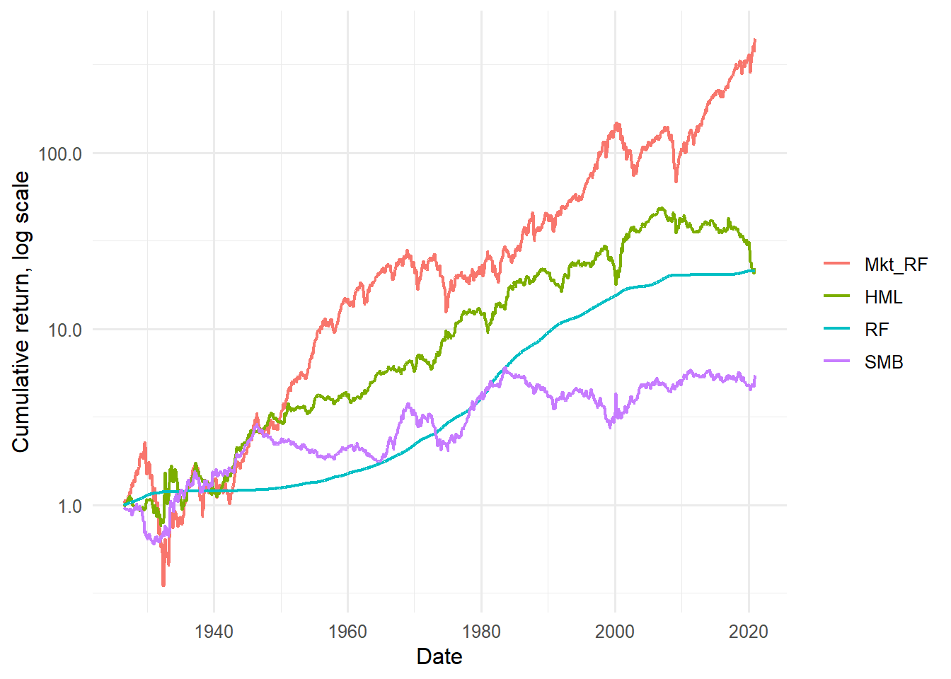
Figure 4.1: Cumulative returns of the Fama-French three factors.
The cumulative-return plot emphasizes that factor premia are earned through time, with long expansions and reversals. A factor can have a positive average return and still experience long drawdowns, so the time path is part of the economic story.
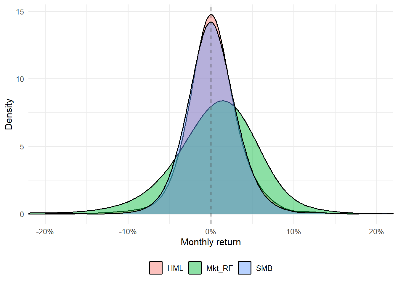
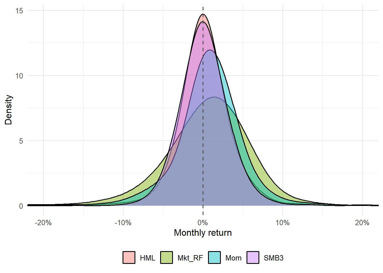
Figure 4.2: Distribution of monthly returns for the Fama-French three factors.
The density plot complements the cumulative plot. It shows where monthly returns are concentrated and how far negative or positive observations can extend. This helps students read factor performance as both a distribution of monthly outcomes and an annualized average.
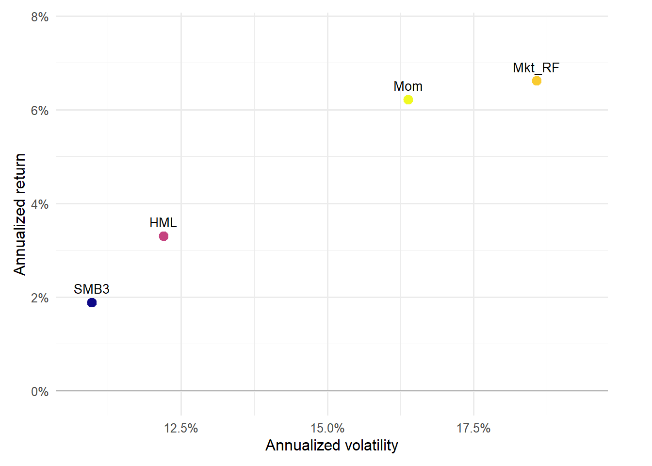
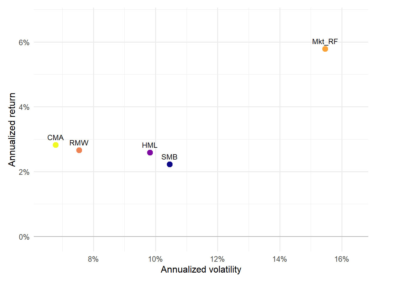
Figure 4.3: Risk-return profile of the factor portfolios.
The risk-return profile compresses the table into one visual comparison. Points higher on the vertical axis have larger annualized returns, while points farther right have higher annualized volatility. Labels make clear which factor drives each position, so the graph can be read as a map of factor rewards and risks.
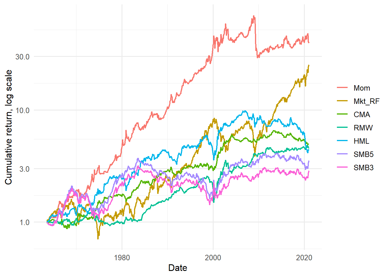
Cumulative factor returns show that factors are portfolios through time. The line for each factor is the wealth path from investing one dollar in that long-short factor portfolio:
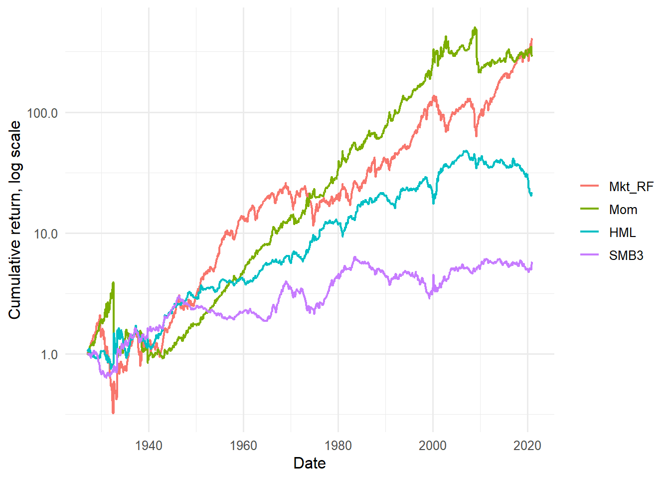
Figure 4.4: Cumulative returns of Fama-French factors and momentum.
Adding momentum changes the visual comparison because the set of candidate factor portfolios is now broader. The purpose of the figure is to show how the market, size, value, and momentum factor histories differ before any asset pricing regression uses them as explanatory variables.
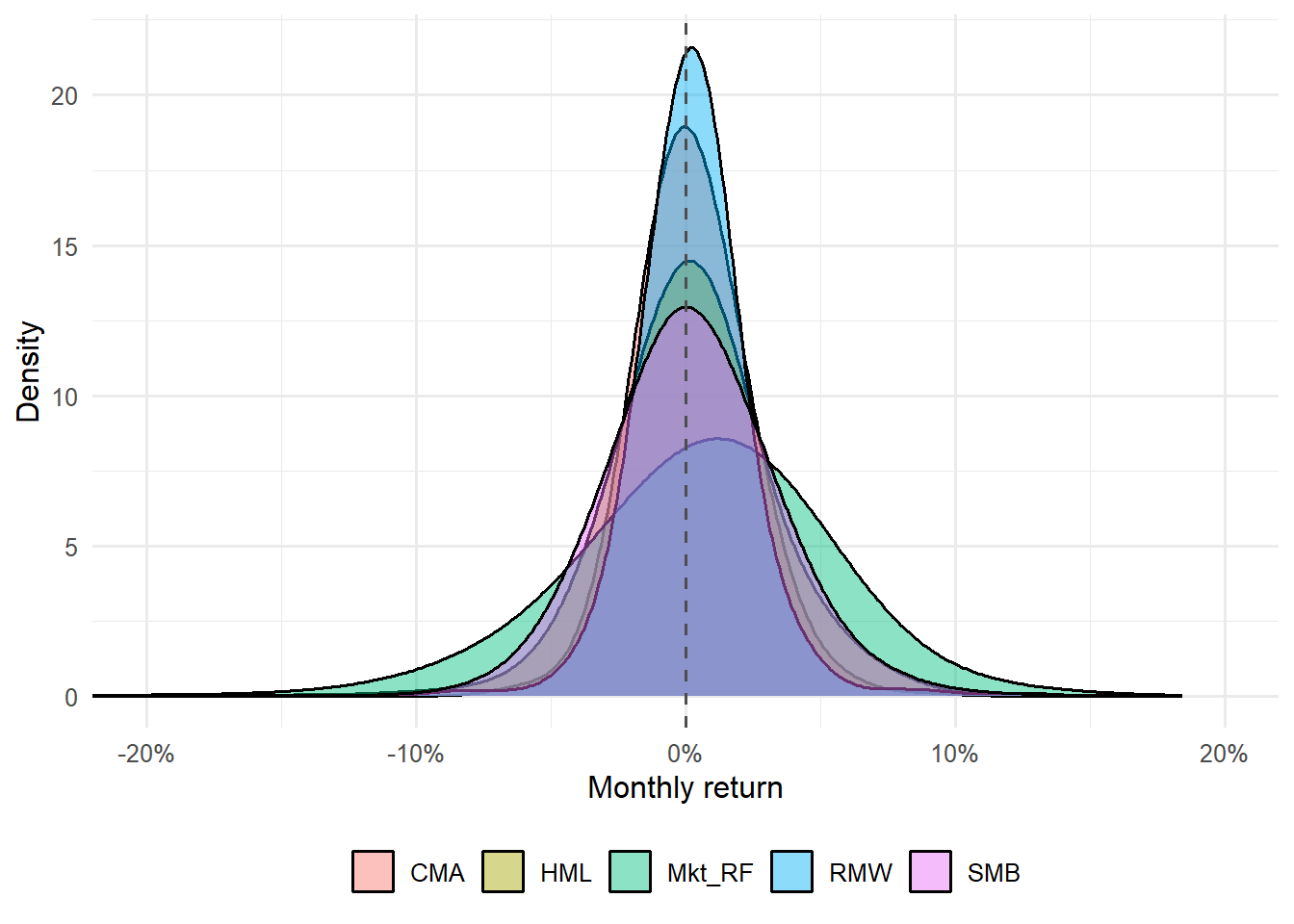
The distribution of monthly factor returns is another diagnostic. Momentum and value can have long episodes of strong performance and sharp reversals, so a factor’s average return should always be read together with its volatility and tail behavior.
Figure 4.5: Distribution of monthly factor returns.
The monthly distributions also show why factor regressions can be sensitive to large episodes. A factor with a similar average return can have a different tail profile, and that affects how individual assets load on it in a regression.
The same workflow can be applied to the five-factor data. The shorter sample starts in 1963, because the profitability and investment factors are available from that point in the downloaded file.
Code
ff5_perf <-annualized_performance(ff5, c("Mkt_RF", "SMB", "HML", "RMW", "CMA"))ff5_perf |>mutate(across(c(annualized_return, annualized_volatility, return_per_unit_risk), ~round(.x, 4))) |>kable(caption ="Annualized performance of the Fama-French five factors.",row.names =FALSE ) |>kable_styling(latex_options ="HOLD_position")
Annualized performance of the Fama-French five factors.
factor
months
annualized_return
annualized_volatility
return_per_unit_risk
SMB
690
0.0222
0.1046
0.2128
HML
690
0.0259
0.0982
0.2636
RMW
690
0.0266
0.0754
0.3534
Mkt_RF
690
0.0578
0.1547
0.3740
CMA
690
0.0283
0.0678
0.4169
The five-factor table prepares the reader for a different factor set and a shorter historical window. Profitability and investment are interpreted as additional dimensions of systematic risk, so their return and volatility should be inspected before they are added to any regression.
The workflow also inspects the five-factor sample and the combined factor set with momentum. The samples differ: the five-factor data start later, and the SMB factor in the five-factor file is a different constructed series from the SMB factor in the three-factor file. The chapter keeps the variable names SMB3 and SMB5 to make that distinction visible in the code.
Annualized performance of the combined factor set.
factor
months
annualized_return
annualized_volatility
return_per_unit_risk
SMB3
690
0.0186
0.1048
0.1772
SMB5
690
0.0222
0.1046
0.2128
HML
690
0.0259
0.0982
0.2636
RMW
690
0.0266
0.0754
0.3534
Mkt_RF
690
0.0578
0.1547
0.3740
CMA
690
0.0283
0.0678
0.4169
Mom
690
0.0661
0.1459
0.4529
The combined table is mainly a bookkeeping and comparison device. It gathers all factor candidates used later in the chapter and makes the sample change visible. A model with more factors is easier to estimate mechanically, but the reader still needs to know which factor histories are being compared.
Figure 4.6: Risk-return profile of the Fama-French five factors.
The five-factor risk-return graph shows whether the added profitability and investment factors occupy distinct positions relative to market, size, and value. If two factors have similar risk-return profiles, the regression may still distinguish them through covariance with asset returns.
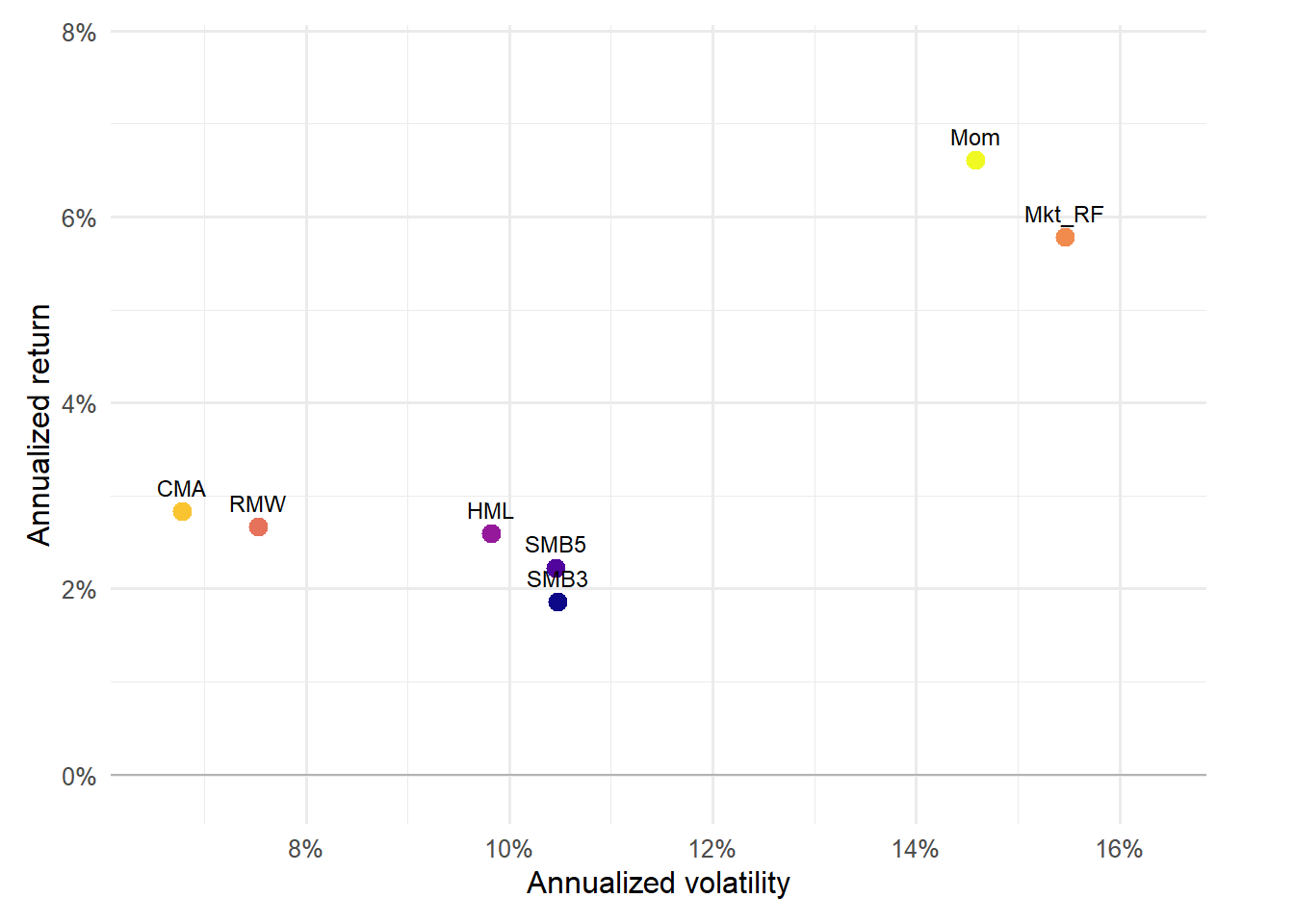
Figure 4.7: Risk-return profile of all factors used in the chapter.
The all-factor graph is the broadest factor map in the chapter. It summarizes the candidate explanatory variables before the chapter turns to test assets, where these factor histories become regressors.
Figure 4.8: Cumulative returns of the Fama-French five factors.
The cumulative five-factor plot lets the reader compare the newer factors in their available sample. The shorter window should be kept in mind when comparing these paths with the earlier three-factor histories.
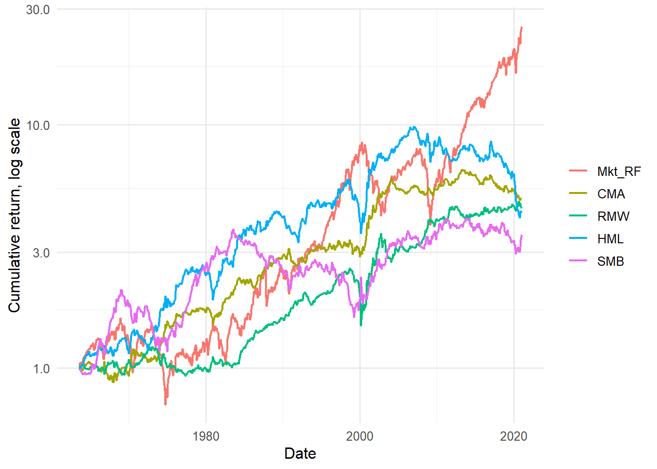
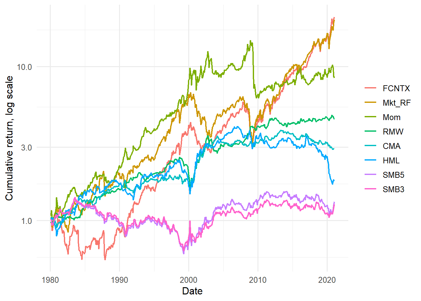
Figure 4.9: Cumulative returns of all factors used in the chapter.
The cumulative all-factor figure is useful for seeing which factors dominate visually and which have more modest paths. This is a descriptive step; the regression step later asks whether these paths help explain asset returns.
Figure 4.10: Distribution of monthly returns for the Fama-French five factors.
The five-factor density plot shows how each factor behaves month by month. Students should read it together with the cumulative plot: the same factor can look attractive cumulatively while still having large monthly downside episodes.
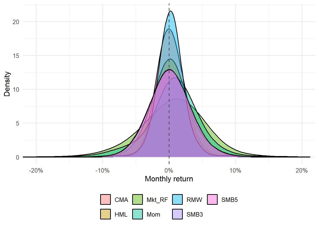
Figure 4.11: Distribution of monthly returns for all factors used in the chapter.
The final factor-density plot closes the descriptive block. At this point, the reader has seen factor returns as tables, cumulative paths, risk-return points, and monthly distributions. The next step is to use those factor returns to explain the behavior of test assets.
4.5 Test assets and the size-value portfolios
The chapter uses two kinds of test assets. The first is FCNTX, a single mutual fund. The second is the 25 Fama-French size-value portfolios. The single asset is useful for seeing one regression closely. The 25 portfolios are useful for testing whether the model explains a structured cross-section of returns.
This table is the first bridge between an individual asset and the factor data. The column returns is the raw FCNTX return, while Re subtracts the risk-free rate. The regression will use Re as the dependent variable and factor returns as explanatory variables, so this joined table is the dataset for the first asset-pricing exercise.
The single-asset exercise checks the data before estimating the regression. The price table verifies the adjusted series used to compute returns. The return table verifies the monthly transformation. The joined table verifies that the excess return and factors are aligned at month end. Reading the three tables in order shows exactly how a price series becomes the dependent variable in the CAPM regression.
Code
first_last_rows(fund_prices) |>select(symbol, date, adjusted) |>kable(caption ="First and last FCNTX adjusted-price observations.",digits =6,row.names =FALSE ) |>kable_styling(latex_options ="HOLD_position")
First and last FCNTX adjusted-price observations.
symbol
date
adjusted
FCNTX
1980-01-02
0.106178
FCNTX
1980-01-03
0.104777
FCNTX
1980-01-04
0.106365
FCNTX
2020-12-28
11.760648
FCNTX
2020-12-29
11.760648
FCNTX
2020-12-30
11.739572
Code
first_last_rows(fund_returns) |>kable(caption ="First and last FCNTX monthly raw returns.",digits =6,row.names =FALSE ) |>kable_styling(latex_options ="HOLD_position")
First and last FCNTX monthly raw returns.
symbol
date
returns
FCNTX
1980-01-31
-0.009675
FCNTX
1980-02-29
-0.016874
FCNTX
1980-03-31
-0.089431
FCNTX
2020-10-30
-0.031775
FCNTX
2020-11-30
0.083591
FCNTX
2020-12-30
0.027920
Code
first_last_rows(fund_factors) |>select(symbol, date, returns, Re, Mkt_RF, SMB3, HML, Mom, SMB5, RMW, CMA, RF) |>kable(caption ="First and last FCNTX excess returns joined to all factors.",digits =6,row.names =FALSE ) |>kable_styling(latex_options ="HOLD_position")
First and last FCNTX excess returns joined to all factors.
symbol
date
returns
Re
Mkt_RF
SMB3
HML
Mom
SMB5
RMW
CMA
RF
FCNTX
1980-01-31
-0.009675
-0.017675
0.0550
0.0162
0.0185
0.0745
0.0188
-0.0184
0.0189
0.0080
FCNTX
1980-02-29
-0.016874
-0.025774
-0.0123
-0.0186
0.0059
0.0789
-0.0162
-0.0095
0.0292
0.0089
FCNTX
1980-03-31
-0.089431
-0.101531
-0.1290
-0.0670
-0.0096
-0.0958
-0.0697
0.0182
-0.0105
0.0121
FCNTX
2020-10-31
-0.031775
-0.031875
-0.0208
0.0434
0.0425
-0.0314
0.0467
-0.0077
-0.0057
0.0001
FCNTX
2020-11-30
0.083591
0.083491
0.1245
0.0581
0.0209
-0.1255
0.0712
-0.0225
0.0128
0.0001
FCNTX
2020-12-31
0.027920
0.027820
0.0463
0.0501
-0.0168
-0.0237
0.0493
-0.0197
-0.0006
0.0001
Code
first_last_rows(portfolio_factor_data) |>select(date, symbol, returns, Re, Mkt_RF, SMB3, HML, Mom) |>kable(caption ="First and last 25-portfolio excess-return rows joined to FF3 and momentum.",digits =6,row.names =FALSE ) |>kable_styling(latex_options ="HOLD_position")
First and last 25-portfolio excess-return rows joined to FF3 and momentum.
date
symbol
returns
Re
Mkt_RF
SMB3
HML
Mom
1927-01-31
SMALL LoBM
0.010954
0.008454
-0.0005
-0.0032
0.0458
0.0057
1927-01-31
ME1 BM2
-0.081352
-0.083852
-0.0005
-0.0032
0.0458
0.0057
1927-01-31
ME1 BM3
-0.048280
-0.050780
-0.0005
-0.0032
0.0458
0.0057
2020-12-31
ME5 BM3
0.034491
0.034391
0.0463
0.0501
-0.0168
-0.0237
2020-12-31
ME5 BM4
0.032226
0.032126
0.0463
0.0501
-0.0168
-0.0237
2020-12-31
BIG HiBM
0.080558
0.080458
0.0463
0.0501
-0.0168
-0.0237
Code
first_last_rows(portfolio_all_factor_data) |>select(date, symbol, returns, Re, Mkt_RF, SMB3, HML, Mom, SMB5, RMW, CMA) |>kable(caption ="First and last 25-portfolio excess-return rows joined to the expanded factor set.",digits =6,row.names =FALSE ) |>kable_styling(latex_options ="HOLD_position")
First and last 25-portfolio excess-return rows joined to the expanded factor set.
date
symbol
returns
Re
Mkt_RF
SMB3
HML
Mom
SMB5
RMW
CMA
1963-07-31
SMALL LoBM
0.011287
0.008587
-0.0039
-0.0057
-0.0081
0.0101
-0.0048
0.0064
-0.0115
1963-07-31
ME1 BM2
-0.003632
-0.006332
-0.0039
-0.0057
-0.0081
0.0101
-0.0048
0.0064
-0.0115
1963-07-31
ME1 BM3
0.007223
0.004523
-0.0039
-0.0057
-0.0081
0.0101
-0.0048
0.0064
-0.0115
2020-12-31
ME5 BM3
0.034491
0.034391
0.0463
0.0501
-0.0168
-0.0237
0.0493
-0.0197
-0.0006
2020-12-31
ME5 BM4
0.032226
0.032126
0.0463
0.0501
-0.0168
-0.0237
0.0493
-0.0197
-0.0006
2020-12-31
BIG HiBM
0.080558
0.080458
0.0463
0.0501
-0.0168
-0.0237
0.0493
-0.0197
-0.0006
The sequence of data checks has a simple logic. First, prices become monthly returns. Second, raw returns become excess returns. Third, each excess return is matched to factor returns for the same month. The 25-portfolio checks repeat the same process for many test assets at once.
Annualized performance of FCNTX excess returns and the factors.
factor
months
annualized_return
annualized_volatility
return_per_unit_risk
SMB3
492
0.0060
0.1026
0.0584
SMB5
492
0.0069
0.1002
0.0690
HML
492
0.0145
0.1031
0.1407
Mom
492
0.0535
0.1558
0.3433
CMA
492
0.0266
0.0676
0.3929
RMW
492
0.0376
0.0818
0.4599
FCNTX
492
0.0771
0.1607
0.4798
Mkt_RF
492
0.0762
0.1561
0.4879
The FCNTX performance table places the mutual fund and factor portfolios on the same scale. This helps answer a descriptive question before estimation: does the fund look more volatile, less volatile, or more rewarded per unit of risk than the factors used to explain it?
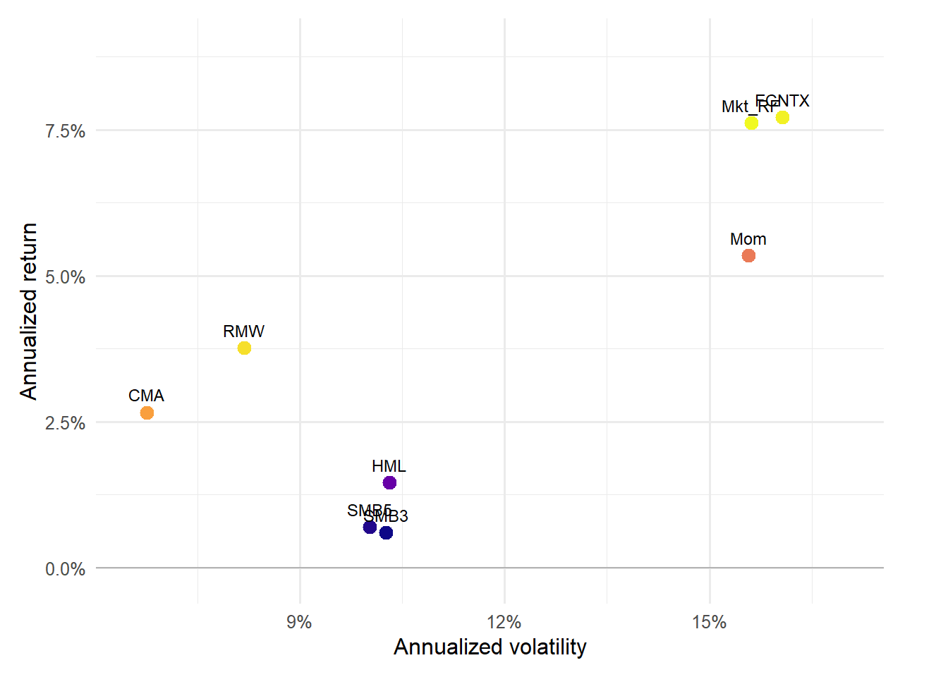
Figure 4.12: Risk-return profile of FCNTX excess returns and the factors.
The risk-return figure makes the same comparison visually. FCNTX appears as one point among the factor portfolios, which helps the reader see whether the fund is close to market-like behavior or whether it sits in a different region of the return-risk space.
Figure 4.13: Cumulative excess returns of FCNTX and the factor portfolios.
The cumulative plot turns the FCNTX comparison into a time-series story. A fund can have a similar average return to a factor while following a different path through time. That difference is exactly what the regression tries to summarize with an intercept, beta, and residual.
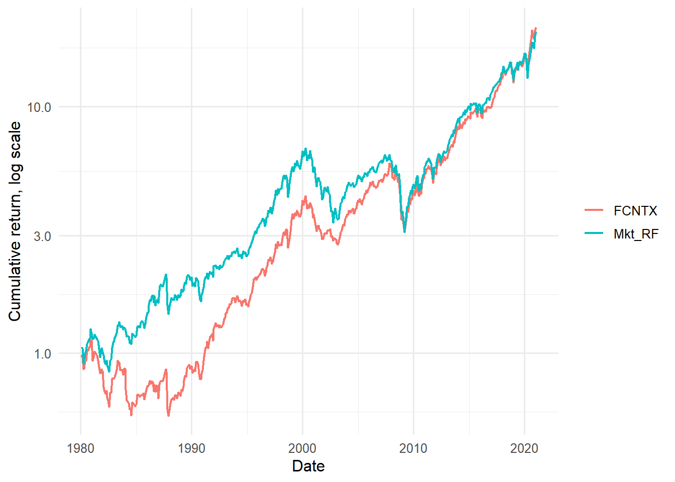
Figure 4.14: Cumulative excess returns of FCNTX and the market factor.
The market comparison isolates the CAPM idea. If FCNTX is mostly a market-risk asset, the FCNTX and market excess-return paths should move together in broad strokes. Differences between the paths foreshadow the residual component in the CAPM regression.
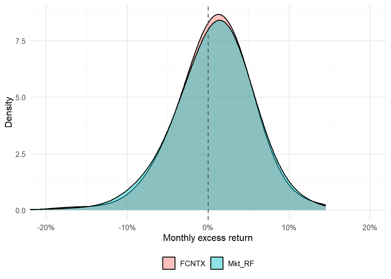
Figure 4.15: Distribution of monthly excess returns for FCNTX and the market factor.
The distribution plot adds another view of the same comparison. Overlap in the two densities suggests similar monthly-return behavior, while differences in spread or tails suggest that market exposure alone may leave unexplained variation.
The single-asset FCNTX example is useful because one regression can be read closely from beginning to end. The 25 Fama-French portfolios serve a different purpose: they create a structured cross-section. Each portfolio is formed by sorting firms by size and book-to-market, so the resulting grid gives the factor model a more demanding asset-pricing problem. The empirical task is now cross-sectional: explain systematic differences across size and value cells.
The same 25 portfolios can be read as investment portfolios through the usual risk-return lens. Annualized return, annualized volatility, and return per unit of risk show the economic content of the size-value grid. Each cell is a portfolio with its own average return and volatility.
Lowest and highest return-risk ratios among the 25 size-value portfolios.
symbol
annualized_return
annualized_volatility
return_per_unit_risk
SMALL LoBM
0.0294
0.4171
0.0705
ME1 BM2
0.0668
0.3380
0.1977
ME2 BM1
0.0795
0.2766
0.2876
BIG HiBM
0.1069
0.2957
0.3615
ME1 BM3
0.1143
0.3092
0.3697
ME5 BM3
0.1047
0.1944
0.5385
BIG LoBM
0.1006
0.1846
0.5447
ME3 BM2
0.1248
0.2253
0.5538
ME3 BM4
0.1345
0.2410
0.5582
ME3 BM3
0.1261
0.2247
0.5611
The table shows the extremes of the 25-portfolio risk-return ranking. This is a compact way to see that the size-value grid contains meaningful heterogeneity: some portfolios deliver much more return per unit of volatility than others.
Code
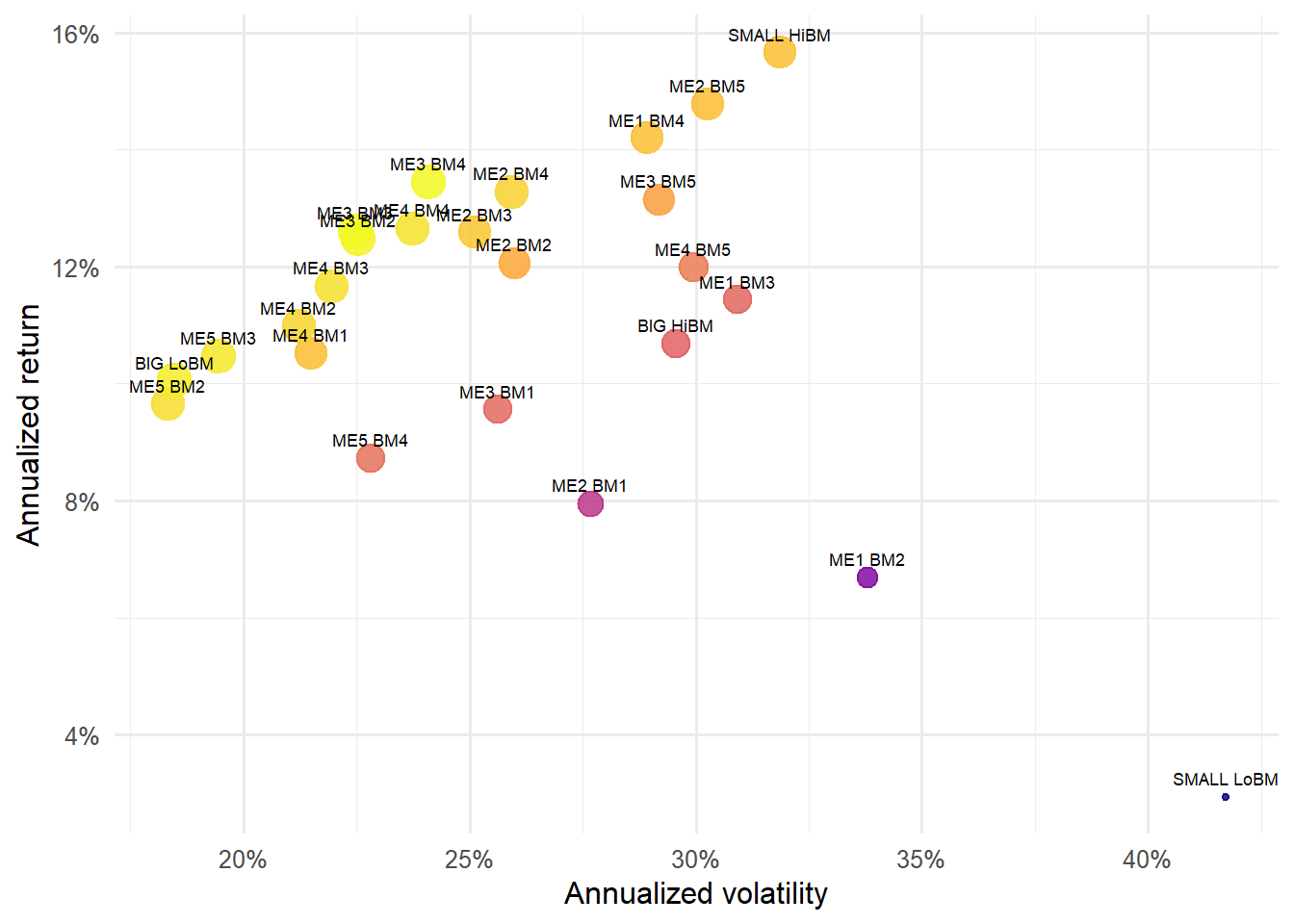
portfolio_perf |>ggplot(aes(annualized_volatility, annualized_return, color = return_per_unit_risk)) +geom_point(aes(size = return_per_unit_risk), alpha =0.85, show.legend =FALSE) +geom_text(aes(label = symbol), vjust =-0.9, size =2.4, color ="black") +labs(x ="Annualized volatility",y ="Annualized return",color ="Return per unit of risk" ) +scale_x_continuous(labels = scales::percent) +scale_y_continuous(labels = scales::percent) +scale_color_viridis_c(option ="C") +theme_minimal(base_size =12) +theme(legend.position ="bottom")
Figure 4.16: Risk-return profile of the 25 size-value portfolios.
The risk-return scatter makes the heterogeneity visible across all 25 portfolios. Dense labels are intentional here because each point is a named test asset. The graph prepares the reader for the asset-pricing question: can factor exposures explain why these portfolios occupy different locations?
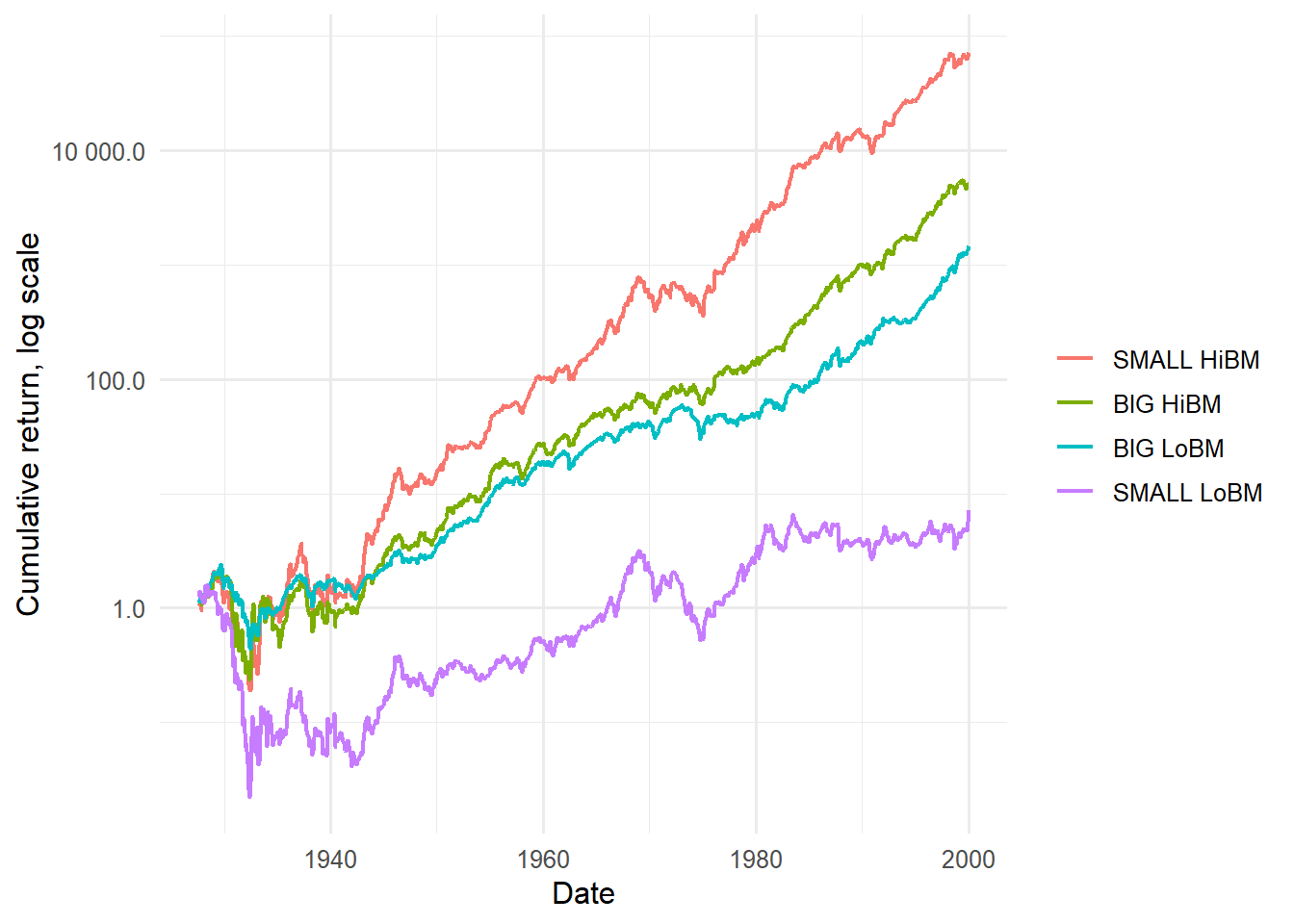
Kenneth French’s data library often illustrates the extreme size-value portfolios because they make the empirical pattern easy to see. The plot below keeps the four corner portfolios: small growth, small value, big growth, and big value.
Figure 4.17: Cumulative raw returns for the four corner size-value portfolios.
The four-corner cumulative plot focuses on the most interpretable cells of the grid. Comparing small versus big and low versus high book-to-market portfolios shows why the size-value sort became a standard test bed for factor models.
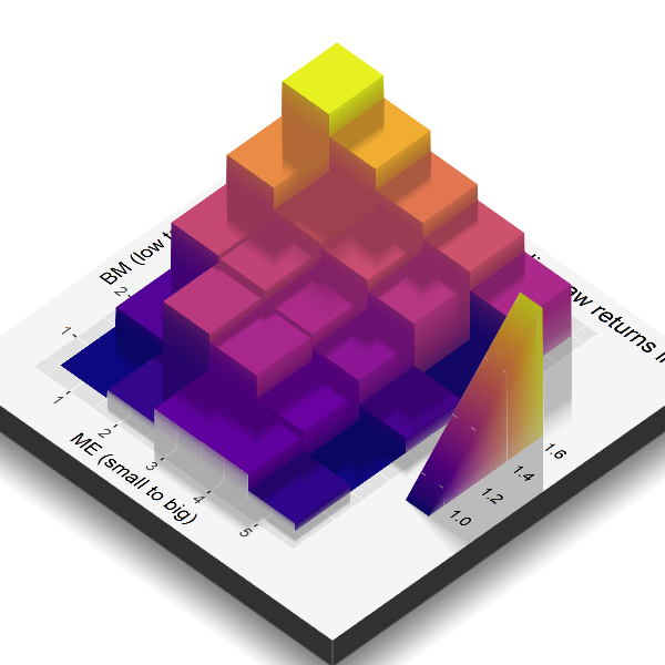
The rendered 3D surface gives a second view of the same size-value grid. The height and color of each cell represent the average monthly raw return of that portfolio.
Mean monthly raw returns behind the size-value surface.
ME
BM1 low
BM2
BM3
BM4
BM5 high
ME1 small
0.8830
0.9688
1.2728
1.4296
1.5976
ME2
0.9524
1.2231
1.2415
1.3062
1.5142
ME3
1.0306
1.1965
1.1989
1.2863
1.3704
ME4
1.0321
1.0570
1.1196
1.2225
1.3006
ME5 big
0.9443
0.9099
0.9878
0.9115
1.1976
The surface table gives the numeric values behind the rendered image. It is the same information in tabular form: rows move from small to big firms, columns move from low to high book-to-market firms, and each entry is the average monthly raw return in percent for that cell.
Figure 4.18: Rendered surface of the 25 size-value portfolio mean returns.
The rendered surface is a visual summary of the size-value pattern. Peaks mark cells with higher average monthly returns; lower blocks mark cells with lower average returns. The point of the figure is to make the cross-sectional pattern visible before the regression tries to explain it with factor exposures.
Animated rendered surface of the 25 size-value portfolio mean returns.
The animation rotates the same surface. It uses the same data and helps the reader see the three-dimensional structure of the 25 portfolio averages.
4.6 Time-series asset pricing regressions
The time-series regression estimates factor exposures for each asset. It uses many months of returns for one asset at a time and asks how that asset moves with the factors. In matrix form, for asset \(i\) and \(K\) factors,
This equation has two roles. The slope vector \(\boldsymbol{\beta}_i\) measures exposure to systematic risk. A high market beta means that the asset tends to rise more in strong market months and fall more in weak market months. A high value beta means that the asset tends to move with the HML factor. The intercept \(\alpha_i\) measures the average excess return that remains after the factor exposures have been used.
The residual \(\varepsilon_{i,t}\) is a month-by-month error. It measures the difference between the observed excess return in month \(t\) and the fitted value from the regression. The alpha is different because it is constant over the sample. It measures an average level left after the factors are included. This distinction is useful: residuals diagnose short-run fit, while alphas diagnose average pricing.
In regression-based asset pricing, alpha is read as a pricing error when the factors are traded return portfolios. A model that prices the asset well should leave a small alpha, because the asset’s average excess return should be accounted for by its factor exposures. For one asset, the alpha tells us what the model leaves unexplained for that asset. For the 25 portfolios, the collection of alphas is more informative: a pattern of large positive and negative alphas would show that the model misses a systematic part of the cross-section.
The regression is therefore doing two jobs at once. Statistically, it is a least-squares fit of returns on factors. Economically, it is asking whether the factor model has removed the average return that should be explained by risk exposure. Cochrane’s regression tests use this second reading: the intercept is evidence about whether the model prices the asset.
The code below wraps that equation in a reusable function. The formula defines the right-hand side. The grouping variable symbol defines which asset receives its own regression.
The code follows the equation in four steps. First, group_by(symbol) separates the data by asset. Second, lm(formula, data = .x) estimates one time-series regression for that asset. Third, broom::tidy() extracts the estimated intercept and betas. Fourth, broom::augment() returns fitted values and residuals month by month. These four objects correspond directly to the mathematical notation: coefficients, fitted values, residuals, and model diagnostics.
fund_capm <-fit_factor_model(fund_factors, Re ~ Mkt_RF)tidy_factor_model(fund_capm) |>mutate(across(where(is.numeric), ~round(.x, 6))) |>kable(caption ="CAPM time-series regression for FCNTX.",row.names =FALSE ) |>kable_styling(latex_options ="HOLD_position")
CAPM time-series regression for FCNTX.
symbol
term
estimate
std.error
statistic
p.value
FCNTX
(Intercept)
0.000766
0.000977
0.783862
0.4335
FCNTX
Mkt_RF
0.913507
0.021423
42.641809
0.0000
The CAPM table has two central entries. The market coefficient is the estimated market beta of FCNTX: it measures how much the fund’s excess return changes with the market excess return. The intercept is the fund’s average excess return after controlling for market exposure. A positive intercept means that FCNTX earned more, on average, than the CAPM would assign from its market beta over this sample. A negative intercept means that the market exposure assigns more average excess return than the fund actually earned.
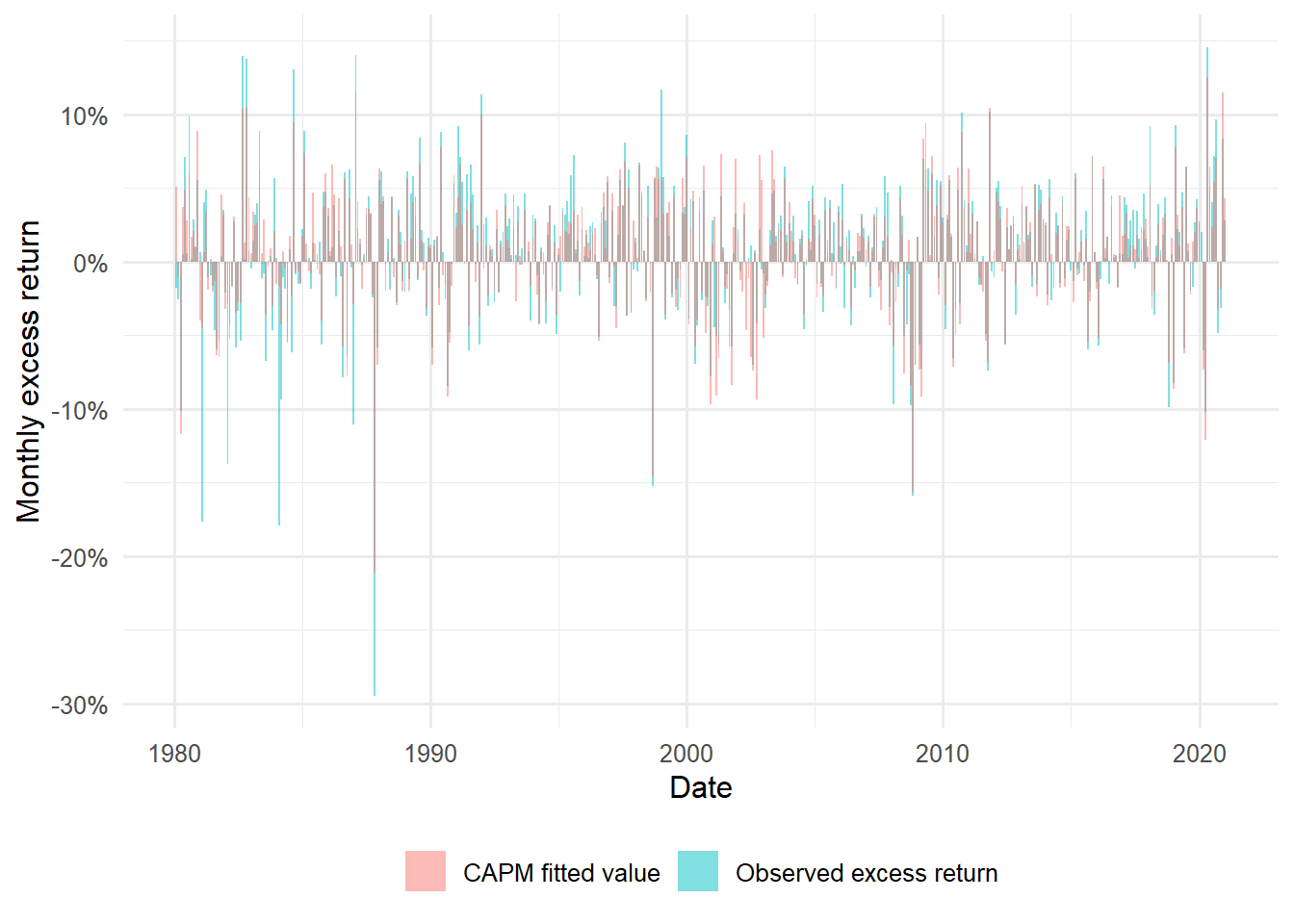
The fitted value is the model-implied excess return for each month:
augment_factor_model(fund_capm) |>ggplot(aes(date)) +geom_col(aes(y = Re, fill ="Observed excess return"), alpha =0.5) +geom_col(aes(y = .fitted, fill ="CAPM fitted value"), alpha =0.5) +labs(x ="Date", y ="Monthly excess return", fill =NULL) +scale_y_continuous(labels = scales::percent) +theme_minimal(base_size =12) +theme(legend.position ="bottom")
Figure 4.19: FCNTX excess returns and CAPM fitted values.
The fitted-value plot shows the CAPM as a month-by-month approximation. Months where the fitted bars and observed bars are close are months where market exposure explains much of the fund’s movement. Large gaps are residuals: the part of the FCNTX excess return left after the market factor is used.
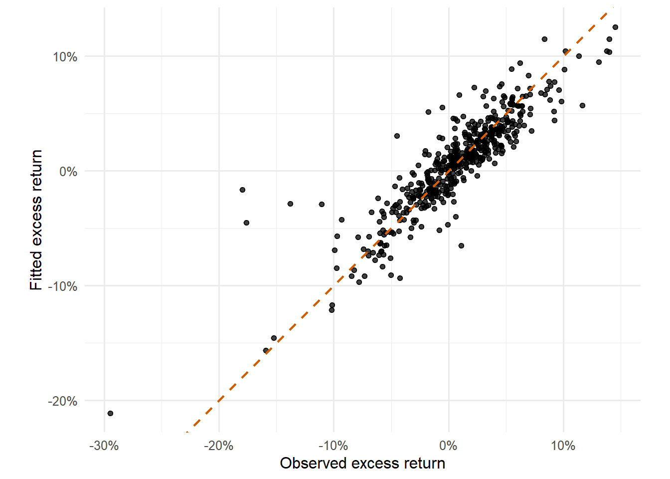
The next graphs check whether the fitted values and residuals look reasonable. They are diagnostics for the time-series fit. They ask whether the CAPM regression is fitting the single asset in a stable way before the chapter moves to the 25-portfolio cross-section.
Figure 4.20: Observed and fitted FCNTX excess returns.
The observed-versus-fitted scatter compresses the time-series fit into one plane. Points near the 45-degree line indicate months where the CAPM fitted return is close to the observed FCNTX excess return. The spread around the line shows the size of month-level errors.
Code
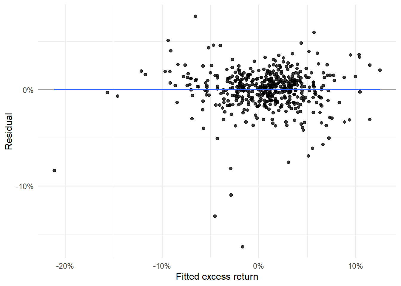
fund_capm_aug |>ggplot(aes(.fitted, .resid)) +geom_hline(yintercept =0, color ="gray60", linewidth =0.5) +geom_point(alpha =0.75) +geom_smooth(method ="lm", formula = y ~ x, se =FALSE, linewidth =0.8) +labs(x ="Fitted excess return", y ="Residual") +scale_x_continuous(labels = scales::percent) +scale_y_continuous(labels = scales::percent) +theme_minimal(base_size =12)
Figure 4.21: FCNTX residuals against fitted values.
The residuals-against-fitted graph checks whether errors change systematically with the fitted return. A visible slope or curved pattern would suggest that the single market factor is leaving structure in the residuals.
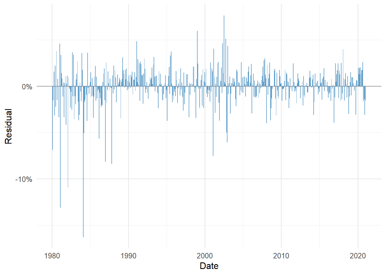
The residual time plot shows whether unexplained returns cluster in particular periods. Clusters are informative because they suggest that the model misses episodes where FCNTX behaves differently from the market factor.
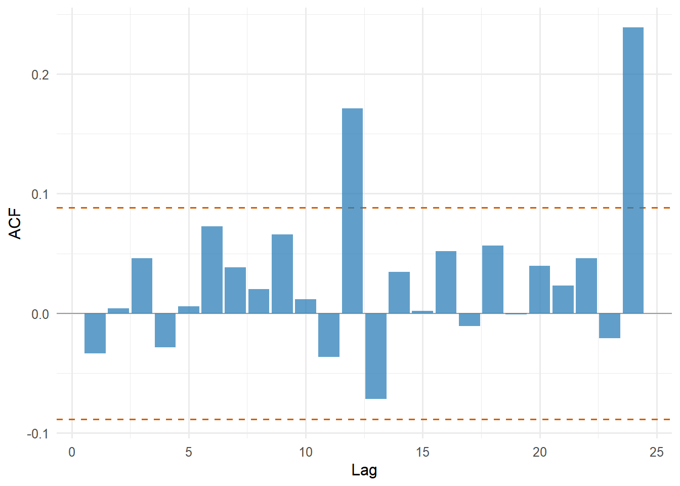
Figure 4.23: Autocorrelation function for FCNTX CAPM residuals.
The autocorrelation plot asks whether residuals are serially related. In a clean time-series regression, residuals should have little predictable structure across lags. Large bars would indicate persistence in the unexplained component.
Code
fund_capm_aug |>group_by(symbol) |>summarise(ljung_box_p_value =Box.test(.resid, lag =10, type ="Ljung-Box", fitdf =2)$p.value,box_pierce_p_value =Box.test(.resid, lag =10, type ="Box-Pierce", fitdf =2)$p.value,.groups ="drop" ) |>mutate(across(where(is.numeric), ~round(.x, 6))) |>kable(caption ="Residual autocorrelation checks for the FCNTX CAPM regression.",row.names =FALSE ) |>kable_styling(latex_options ="HOLD_position")
Residual autocorrelation checks for the FCNTX CAPM regression.
symbol
ljung_box_p_value
box_pierce_p_value
FCNTX
0.446524
0.459502
The Ljung-Box and Box-Pierce p-values formalize the residual-autocorrelation check. They summarize whether residual autocorrelation is large enough to be a statistical concern at the chosen lag.
For the 25 portfolios, the CAPM estimates 25 market betas:
Code
portfolio_capm <-fit_factor_model(portfolio_factor_data, Re ~ Mkt_RF)tidy_factor_model(portfolio_capm) |>filter(term =="Mkt_RF") |>arrange(estimate) |>slice(c(1:5, (n() -4):n())) |>mutate(across(where(is.numeric), ~round(.x, 6))) |>kable(caption ="Lowest and highest CAPM market betas among the 25 portfolios.",row.names =FALSE ) |>kable_styling(latex_options ="HOLD_position")
Lowest and highest CAPM market betas among the 25 portfolios.
symbol
term
estimate
std.error
statistic
p.value
ME5 BM2
Mkt_RF
0.948845
0.008293
114.41417
0
BIG LoBM
Mkt_RF
0.956923
0.008451
113.23358
0
ME5 BM3
Mkt_RF
0.973296
0.011799
82.48904
0
ME4 BM1
Mkt_RF
1.087596
0.012244
88.82592
0
ME4 BM2
Mkt_RF
1.092239
0.010432
104.69953
0
SMALL HiBM
Mkt_RF
1.378264
0.030716
44.87166
0
ME2 BM5
Mkt_RF
1.389511
0.025664
54.14304
0
ME1 BM2
Mkt_RF
1.404849
0.034684
40.50444
0
ME4 BM5
Mkt_RF
1.407824
0.023693
59.42046
0
SMALL LoBM
Mkt_RF
1.612572
0.046799
34.45776
0
The beta table shows the range of market exposures across the 25 portfolios. This range is important because cross-sectional asset pricing needs variation in exposures. If all portfolios had nearly identical market betas, market beta would have little power to explain differences in average returns.
Code
tidy_factor_model(portfolio_capm) |>arrange(symbol, term) |>mutate(across(where(is.numeric), ~round(.x, 6))) |>kable(caption ="CAPM coefficients for all 25 size-value portfolios.",row.names =FALSE ) |>kable_styling(latex_options ="HOLD_position")
CAPM coefficients for all 25 size-value portfolios.
symbol
term
estimate
std.error
statistic
p.value
BIG HiBM
(Intercept)
0.000386
0.001466
0.263512
0.792204
BIG HiBM
Mkt_RF
1.311025
0.027131
48.322346
0.000000
BIG LoBM
(Intercept)
0.000235
0.000457
0.514319
0.607130
BIG LoBM
Mkt_RF
0.956923
0.008451
113.233577
0.000000
ME1 BM2
(Intercept)
-0.002389
0.001874
-1.274688
0.202683
ME1 BM2
Mkt_RF
1.404849
0.034684
40.504445
0.000000
ME1 BM3
(Intercept)
0.000817
0.001540
0.530487
0.595879
ME1 BM3
Mkt_RF
1.370093
0.028504
48.066185
0.000000
ME1 BM4
(Intercept)
0.003006
0.001452
2.070068
0.038674
ME1 BM4
Mkt_RF
1.276523
0.026874
47.499692
0.000000
ME2 BM1
(Intercept)
-0.001812
0.001266
-1.431260
0.152633
ME2 BM1
Mkt_RF
1.272654
0.023426
54.326724
0.000000
ME2 BM2
(Intercept)
0.001222
0.001082
1.129123
0.259087
ME2 BM2
Mkt_RF
1.233511
0.020020
61.613546
0.000000
ME2 BM3
(Intercept)
0.001573
0.001013
1.553653
0.120548
ME2 BM3
Mkt_RF
1.201998
0.018741
64.136138
0.000000
ME2 BM4
(Intercept)
0.002183
0.001097
1.989744
0.046861
ME2 BM4
Mkt_RF
1.222209
0.020303
60.199031
0.000000
ME2 BM5
(Intercept)
0.002979
0.001387
2.148093
0.031919
ME2 BM5
Mkt_RF
1.389511
0.025664
54.143036
0.000000
ME3 BM1
(Intercept)
-0.000804
0.000957
-0.840684
0.400704
ME3 BM1
Mkt_RF
1.251067
0.017708
70.650107
0.000000
ME3 BM2
(Intercept)
0.001550
0.000723
2.143617
0.032277
ME3 BM2
Mkt_RF
1.132414
0.013380
84.637675
0.000000
ME3 BM3
(Intercept)
0.001725
0.000745
2.315546
0.020762
ME3 BM3
Mkt_RF
1.123102
0.013787
81.459133
0.000000
ME3 BM4
(Intercept)
0.002106
0.000907
2.322279
0.020396
ME3 BM4
Mkt_RF
1.174158
0.016781
69.970866
0.000000
ME3 BM5
(Intercept)
0.001745
0.001260
1.384606
0.166447
ME3 BM5
Mkt_RF
1.366313
0.023325
58.577659
0.000000
ME4 BM1
(Intercept)
0.000217
0.000662
0.327664
0.743227
ME4 BM1
Mkt_RF
1.087596
0.012244
88.825923
0.000000
ME4 BM2
(Intercept)
0.000440
0.000564
0.780063
0.435518
ME4 BM2
Mkt_RF
1.092239
0.010432
104.699533
0.000000
ME4 BM3
(Intercept)
0.000989
0.000682
1.449711
0.147417
ME4 BM3
Mkt_RF
1.107003
0.012623
87.695115
0.000000
ME4 BM4
(Intercept)
0.001596
0.000863
1.850184
0.064549
ME4 BM4
Mkt_RF
1.164925
0.015966
72.964317
0.000000
ME4 BM5
(Intercept)
0.000763
0.001280
0.595705
0.551492
ME4 BM5
Mkt_RF
1.407824
0.023693
59.420458
0.000000
ME5 BM2
(Intercept)
-0.000152
0.000448
-0.339499
0.734297
ME5 BM2
Mkt_RF
0.948845
0.008293
114.414172
0.000000
ME5 BM3
(Intercept)
0.000567
0.000638
0.889874
0.373724
ME5 BM3
Mkt_RF
0.973296
0.011799
82.489044
0.000000
ME5 BM4
(Intercept)
-0.001169
0.000868
-1.347608
0.178056
ME5 BM4
Mkt_RF
1.106035
0.016059
68.872918
0.000000
SMALL HiBM
(Intercept)
0.003906
0.001660
2.353169
0.018785
SMALL HiBM
Mkt_RF
1.378264
0.030716
44.871658
0.000000
SMALL LoBM
(Intercept)
-0.004870
0.002529
-1.925603
0.054406
SMALL LoBM
Mkt_RF
1.612572
0.046799
34.457758
0.000000
The full coefficient table keeps the individual portfolio estimates visible. Each portfolio has its own intercept and market beta, so the CAPM is estimated as 25 separate time-series regressions, one for each test asset. The market beta column measures exposure. The intercept column should be read as the CAPM pricing error for each portfolio. If those intercepts are systematically high for one part of the size-value grid and low for another, the CAPM is missing a cross-sectional pattern across many assets.
The 25 separate CAPM regressions have different levels of fit. A compact way to inspect them is to compare \(R^2\), residual standard error, and residual autocorrelation diagnostics across portfolios.
Code
portfolio_capm_diagnostics <-glance_factor_model(portfolio_capm) |>select(symbol, r.squared, adj.r.squared, sigma, AIC, BIC) |>arrange(r.squared)portfolio_capm_diagnostics |>slice(c(1:5, (n() -4):n())) |>mutate(across(where(is.numeric), ~round(.x, 4))) |>kable(caption ="Lowest and highest CAPM goodness-of-fit values among the 25 portfolios.",row.names =FALSE ) |>kable_styling(latex_options ="HOLD_position")
Lowest and highest CAPM goodness-of-fit values among the 25 portfolios.
symbol
r.squared
adj.r.squared
sigma
AIC
BIC
SMALL LoBM
0.5133
0.5128
0.0843
-2375.900
-2360.815
ME1 BM2
0.5930
0.5926
0.0624
-3051.749
-3036.664
SMALL HiBM
0.6413
0.6410
0.0553
-3325.851
-3310.767
ME1 BM4
0.6671
0.6668
0.0484
-3627.258
-3612.173
ME1 BM3
0.6723
0.6720
0.0513
-3494.418
-3479.333
ME4 BM3
0.8723
0.8722
0.0227
-5331.951
-5316.866
ME4 BM1
0.8751
0.8750
0.0220
-5400.756
-5385.671
ME4 BM2
0.9068
0.9068
0.0188
-5762.069
-5746.985
BIG LoBM
0.9193
0.9192
0.0152
-6237.228
-6222.144
ME5 BM2
0.9208
0.9207
0.0149
-6279.753
-6264.668
The goodness-of-fit table shows which portfolios are relatively well described by the market factor and which are less well described. A higher \(R^2\) means that market movements explain a larger fraction of that portfolio’s excess return variation.
Code
augment_factor_model(portfolio_capm) |>group_by(symbol) |>summarise(box_pierce_p_value =Box.test(.resid, lag =10, type ="Box-Pierce", fitdf =2)$p.value,.groups ="drop" ) |>arrange(box_pierce_p_value) |>slice(c(1:5, (n() -4):n())) |>mutate(box_pierce_p_value =round(box_pierce_p_value, 6)) |>kable(caption ="Lowest and highest Box-Pierce p-values for the 25 CAPM residual series.",row.names =FALSE ) |>kable_styling(latex_options ="HOLD_position")
Lowest and highest Box-Pierce p-values for the 25 CAPM residual series.
symbol
box_pierce_p_value
ME3 BM4
0.000000
ME2 BM4
0.000000
SMALL LoBM
0.000000
ME4 BM5
0.000000
ME4 BM2
0.000000
ME3 BM5
0.003763
ME1 BM3
0.008790
ME4 BM1
0.015569
SMALL HiBM
0.043218
ME5 BM2
0.075859
The residual test table extends the diagnostic logic from FCNTX to the full portfolio set. Portfolios with very small p-values deserve attention because their residuals show stronger serial structure under the CAPM specification.
4.7 Asset pricing errors and factor exposures
The Fama-French three-factor model is the main worked example for the rest of the chapter. It is detailed enough to show the full econometric route: first estimate time-series betas, then estimate cross-sectional prices of risk, then compare the beta-method with SDF-GMM estimates. Momentum and the five-factor model appear later as faster extensions. They are useful for comparison, while the main explanation is developed with FF3.
The Fama-French three-factor model adds size and value exposures:
The fitted expected excess return is obtained by taking the estimated factor loadings and multiplying them by average factor returns. The intercept is reported separately because, in asset pricing, alpha is the pricing error:
This equation is the bridge between the regression table and the asset-pricing plot. The regression estimates betas. The asset-pricing restriction asks whether those betas, without an asset-specific alpha, explain average excess returns. If \(\widehat{\alpha}_i\) is economically important, the factor model is leaving a pricing error for asset \(i\).
The distinction is important for interpretation. A time-series regression with an intercept can always decompose the sample average return into two parts:
The term \(\widehat{\boldsymbol{\beta}}_i^\top\bar{\mathbf{f}}\) is the return explained by factor exposures. The term \(\widehat{\alpha}_i\) is the part that remains asset-specific after those exposures have been used. The asset-pricing question is therefore direct: are the alphas small enough for the factor model to be a credible explanation of average returns?
This decomposition comes from averaging the monthly regression over the sample. Start with the fitted regression,
In an ordinary least-squares regression with an intercept, the sample average of the residuals is zero. That is why the average return can be written as alpha plus the factor-implied component. This algebra also explains why a time-series fitted-average plot can look strong: each asset has its own intercept. The stricter asset-pricing question begins when the chapter asks whether the factor exposures alone can organize average returns across many assets through common prices of risk.
The code mirrors the same decomposition. The function expected_return_from_betas() first computes average factor returns, then multiplies them by the estimated betas, then keeps alpha separately. The column factor_implied_percent is \(100\widehat{\boldsymbol{\beta}}_i^\top\bar{\mathbf{f}}\). The column alpha_percent is \(100\widehat{\alpha}_i\). The observed average excess return is the sum of those two pieces, up to rounding.
This code block prepares the data for the figures that follow. It estimates the three-factor model, stores each portfolio’s factor exposures, computes the factor-implied part of average return, and keeps alpha as the remaining asset-specific component.
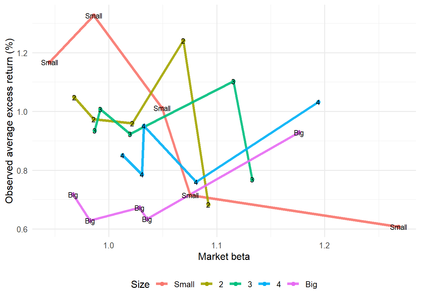
The size and value patterns can be inspected directly by reading average excess returns against market beta by portfolio sort.
The market-beta plots deliberately ignore the fitted-return axis and return to the raw relation between market exposure and average excess returns. If market beta were enough to explain the 25 portfolios, higher beta portfolios would line up with higher average returns in a stable pattern. The size and value groupings show whether portfolios with similar market beta still differ because of their position in the size-value grid.
Code
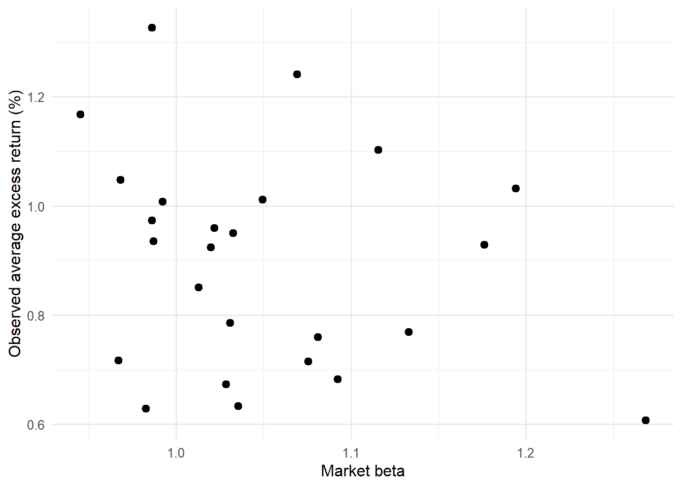
ff3_betas |>filter(term =="Mkt_RF") |>rename(market_beta = estimate) |>select(symbol, market_beta) |>inner_join(ff3_expected, by ="symbol") |>ggplot(aes(market_beta, ERe_percent)) +geom_point(size =2.2) +labs(x ="Market beta", y ="Observed average excess return (%)") +theme_minimal(base_size =12)
Figure 4.24: Market beta and average excess returns for the 25 portfolios.
The plain market-beta graph is the starting point for the anomaly discussion. If market beta alone organized average returns, the cloud would show a clear upward relation. A scattered pattern motivates the size and value groupings in the next two figures.
Code
ff3_betas |>filter(term =="Mkt_RF") |>rename(market_beta = estimate) |>select(symbol, market_beta) |>inner_join(ff3_expected, by ="symbol") |>ggplot(aes(market_beta, ERe_percent, color = Size, group = Size)) +geom_line(alpha =0.9, linewidth =1.5) +geom_point(size =2) +geom_text(aes(label = Size), color ="black", size =3, show.legend =FALSE) +labs(x ="Market beta", y ="Observed average excess return (%)", color ="Size") +theme_minimal(base_size =12) +theme(legend.position ="bottom")
Figure 4.25: Market beta and average excess returns by size portfolio.
The size plot connects each point to its size group. Lines that separate by size indicate that portfolios with similar market beta can have different average returns because they belong to different size cells.
Code
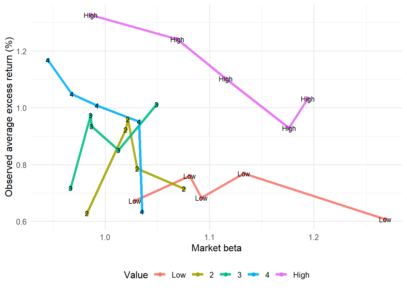
ff3_betas |>filter(term =="Mkt_RF") |>rename(market_beta = estimate) |>select(symbol, market_beta) |>inner_join(ff3_expected, by ="symbol") |>ggplot(aes(market_beta, ERe_percent, color = Value, group = Value)) +geom_line(alpha =0.9, linewidth =1.5) +geom_point(size =2) +geom_text(aes(label = Value), color ="black", size =3, show.legend =FALSE) +labs(x ="Market beta", y ="Observed average excess return (%)", color ="Value") +theme_minimal(base_size =12) +theme(legend.position ="bottom")
Figure 4.26: Market beta and average excess returns by value portfolio.
The value plot reads the same beta-return relation through book-to-market groups. Separation by value group is the visual motivation for adding the HML factor to the model.
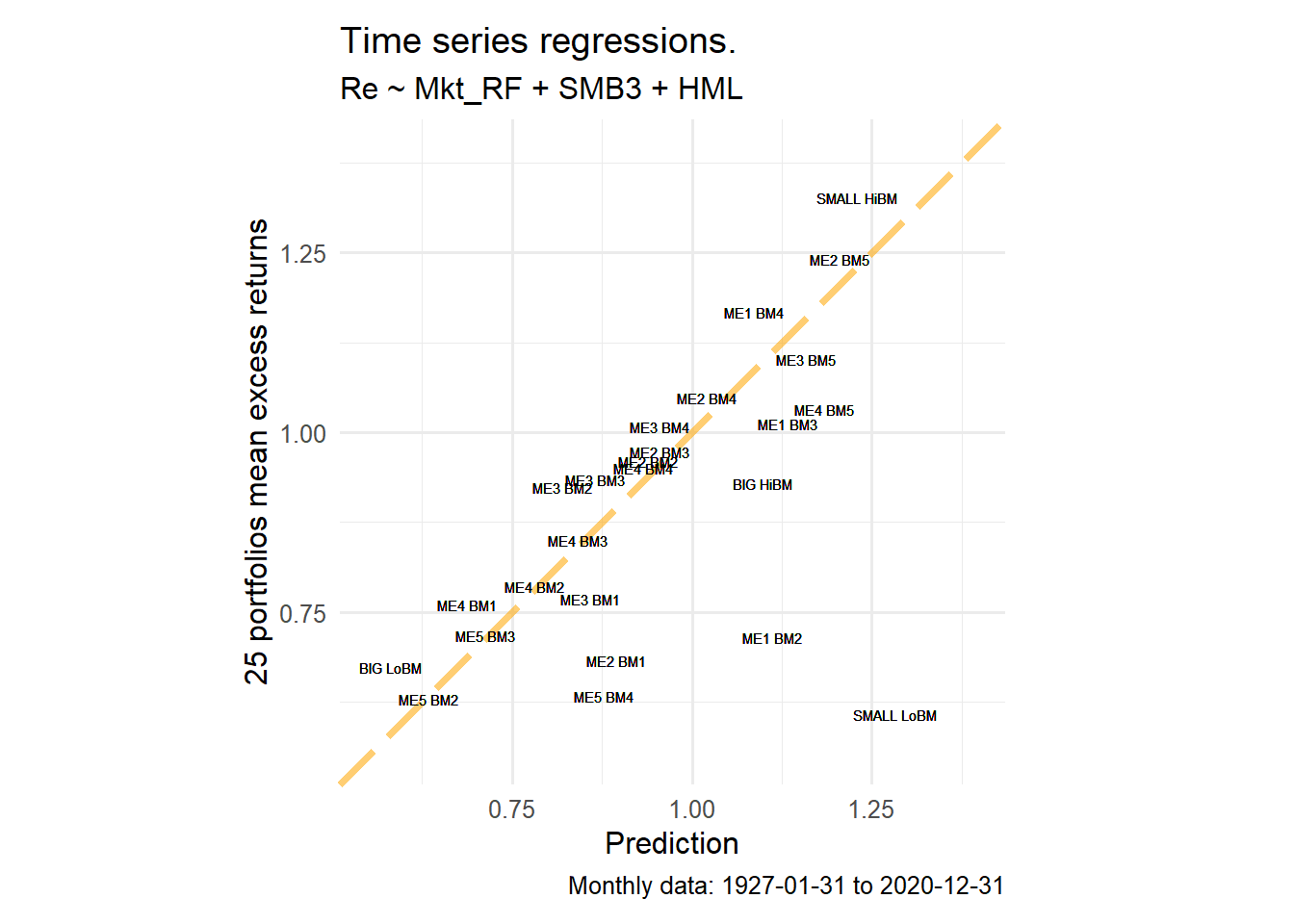
The next diagnostic compares observed average excess returns with predictions assembled from the time-series regression output. This is the last first-pass graph before the chapter moves to cross-sectional pricing. For each portfolio, the regression estimates an intercept and factor loadings. In consistent decimal units, the sample-average decomposition is
These prediction figures should be read as orientation and replication checks. They preserve the display convention of the source FF exercise: average excess returns and factor means are displayed in percent, while the intercept is kept as the coefficient returned by the regression. This convention preserves the numerical values of the FF graphic.
The formal asset-pricing interpretation remains the decimal-unit decomposition above. That equation is the coherent accounting identity: average excess return equals alpha plus the factor-implied component. The figures in this block have a narrower role. They show whether portfolios with high observed average returns also receive high first-pass fitted values before the chapter moves to the stricter cross-sectional pricing test.
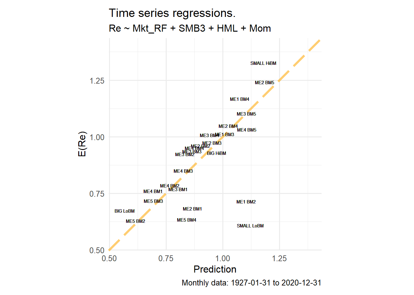
The reading is the same as in the FF3 figure. Adding momentum changes the factor set used to compute the prediction, while the observed average excess return on the vertical axis remains the same portfolio statistic. The figure is a source exercise replication check and a transition to the next section. The cross-sectional test begins after this point, where common prices of risk are estimated across portfolios.
Figure 4.28: Time-series fitted average excess returns under the FF3-plus-momentum model.
The remaining asset-pricing tests use a deliberate division of labor. FF3 is the detailed benchmark. The two extensions are included to show how the results change when the factor set expands.
Code
model_comparison_roadmap <-tibble(model =c("FF3", "FF3 plus momentum", "FF5"),role =c("Detailed benchmark", "Fast comparison", "Fast comparison"),factors =c("Mkt_RF, SMB3, HML","Mkt_RF, SMB3, HML, Mom","Mkt_RF, SMB5, HML, RMW, CMA" ),sample_start =c(min(portfolio_factor_data$date),min(portfolio_factor_data$date),min(portfolio_all_factor_data$date) ),sample_end =c(max(portfolio_factor_data$date),max(portfolio_factor_data$date),max(portfolio_all_factor_data$date) ),months =c(n_distinct(portfolio_factor_data$date),n_distinct(portfolio_factor_data$date),n_distinct(portfolio_all_factor_data$date) ))model_comparison_roadmap |>mutate(across(c(sample_start, sample_end), as.character)) |>kable(caption ="Roadmap for the FF3 benchmark and the comparison models.",row.names =FALSE ) |>kable_styling(latex_options ="HOLD_position")
Roadmap for the FF3 benchmark and the comparison models.
model
role
factors
sample_start
sample_end
months
FF3
Detailed benchmark
Mkt_RF, SMB3, HML
1927-01-31
2020-12-31
1128
FF3 plus momentum
Fast comparison
Mkt_RF, SMB3, HML, Mom
1927-01-31
2020-12-31
1128
FF5
Fast comparison
Mkt_RF, SMB5, HML, RMW, CMA
1963-07-31
2020-12-31
690
The roadmap prevents repetition. FF3 receives the full mathematical and statistical explanation. The momentum and five-factor rows will be read later as robustness comparisons: the same test assets, a different factor set, and a different sample for FF5 because those factors start later.
4.8 Cross-sectional asset pricing tests
Time-series regressions estimate betas. Cross-sectional regressions ask whether those betas explain average returns across assets. The data shape changes at this point. The regression now has one row for each test portfolio. The dependent variable is the portfolio’s average excess return. The explanatory variables are the betas estimated in the previous time-series step.
The intuition is the same as pricing any characteristic. A beta is a quantity of exposure. A lambda is the price attached to that exposure. The fitted value is the total average excess return assigned by the pricing equation after adding up the priced exposures. For a three-factor model, the fitted value is
This equation should be read portfolio by portfolio. A portfolio with high market beta receives more fitted return when \(\widehat{\lambda}_M\) is positive. A portfolio with high value beta receives more fitted return when \(\widehat{\lambda}_H\) is positive. If a beta is high but its lambda is close to zero, that exposure does little work in the fitted cross-section.
This is the expected-return beta representation emphasized in regression-based asset pricing. Cochrane’s chapter 12 frames this equation as a cross-sectional line fitted through test assets (Cochrane 2005). The betas are the right-hand-side variables, the lambdas are the coefficients of the pricing line, and the residuals are pricing errors. The OLS beta-method chooses the lambdas that minimize the sum of squared pricing errors across the 25 portfolios:
This objective explains the visual role of the fitted-return plot. The 45-degree line represents perfect pricing for every test asset. OLS chooses one common pricing equation that brings the points as close as possible to that line in a least-squares sense.
This is a static two-pass cross-sectional regression. It is related to the Fama-MacBeth logic used in asset pricing (Fama and MacBeth 1973), because both approaches first estimate exposures and then price those exposures in a cross-section. A formal Fama-MacBeth procedure would repeat the cross-sectional regression period by period and estimate inference from the time series of price-of-risk estimates. The chapter uses the simpler static version to keep the bridge between betas, prices of risk, fitted returns, and pricing errors transparent. In this chapter, the cross-section is the set of 25 size-value portfolios.
The equation has a clear economic reading. The left-hand side, \(\bar{R}_i^e\), is the average excess return of portfolio \(i\). The regressors are estimated exposures from the first-pass time-series regressions. The coefficients \(\lambda_M\), \(\lambda_S\), and \(\lambda_H\) are prices of risk in the cross-section. A positive \(\lambda_H\) means that, holding market and size exposure fixed, portfolios with higher value exposure have higher average excess returns in this sample. A low fitted value for a portfolio means that its estimated betas explain less than its observed average return under this second-pass equation.
The units are also important. The response variable is measured as average monthly excess return in percent. Therefore a \(\lambda\) coefficient is the change in average monthly excess return, in percentage points, associated with one additional unit of the corresponding beta, holding the other betas fixed. A positive price of risk rewards exposure to that factor in this cross-section. A negative price of risk penalizes that exposure in this sample. A coefficient near zero says that the estimated beta does little to organize average returns once the other betas are included.
The residual \(\eta_i\) is the cross-sectional pricing error. It is the vertical gap between the portfolio’s observed average excess return and the fitted value assigned by the common pricing equation. This gap is different from the time-series residual \(\varepsilon_{i,t}\): \(\varepsilon_{i,t}\) is a month-level error, while \(\eta_i\) is an average-return error for one portfolio.
Cochrane often writes the cross-sectional residual as an alpha. This chapter uses \(\eta_i\) in the cross-sectional equation to keep two objects separate: \(\alpha_i\) is the time-series intercept for asset \(i\), and \(\eta_i\) is the cross-sectional pricing error after the common lambda estimates are applied. Both objects diagnose model fit, but they come from different regressions.
There are therefore two layers of estimation:
Layer
Object estimated
Data orientation
Economic role
Time-series regression
\(\alpha_i\) and \(\boldsymbol{\beta}_i\) for each asset
One asset across many months
Measures exposure to factors
Cross-sectional regression
\(\lambda\) coefficients
Many assets in one average-return cross-section
Prices those exposures
The first layer asks how each portfolio moves with the factors. The second layer asks whether those exposures explain why some portfolios earn higher average excess returns than others.
The important change is the source of the fitted value. In the time-series figures, each portfolio has its own intercept, so each regression can match its own sample average closely. In the cross-sectional regression, the fitted value comes from one common pricing equation shared by the 25 portfolios. A portfolio receives a high fitted average return only if its estimated exposures combine with the estimated prices of risk to justify that return. This is the economic content of the second pass: betas become explanatory variables for average returns.
broom::glance(cross_section_fit) |>mutate(across(where(is.numeric), ~round(.x, 6))) |>kable(caption ="Goodness-of-fit summary for the beta-method cross-sectional regression.",row.names =FALSE ) |>kable_styling(latex_options ="HOLD_position")
Goodness-of-fit summary for the beta-method cross-sectional regression.
r.squared
adj.r.squared
sigma
statistic
p.value
df
logLik
AIC
BIC
deviance
df.residual
nobs
0.654312
0.604928
0.12413
13.24945
4.5e-05
3
18.86654
-27.73308
-21.6387
0.323575
21
25
The cross-sectional block should be read as a second pass. The first table is the data matrix: one row per portfolio, average excess return as the outcome, and estimated betas as regressors. The coefficient table estimates the prices attached to those betas. The goodness-of-fit table summarizes how much of the 25-portfolio average-return pattern is captured by this beta-pricing equation. Reading these tables in order prevents a common confusion. The beta table by itself only reports exposures. The coefficient table tells how the cross-section prices those exposures. The fitted-value plot then translates the estimated pricing equation back into portfolio-level average returns.
The coefficient table should be read in three passes. First, inspect the sign of each \(\lambda\): it tells whether the exposure is rewarded or penalized in this sample. Second, inspect the magnitude: it tells how much the fitted average return changes when the beta changes by one unit. Third, inspect the standard errors and p-values with caution: the betas were estimated in a first pass, so the usual OLS table is an orientation device for inference. This is why the chapter later separates estimation logic from formal inference limits.
In this sample, the beta-method gives a concrete result. The cross-sectional \(R^2\) is 0.65, so the estimated betas capture a substantial part of the 25-portfolio average-return pattern while leaving visible pricing errors. The estimated market price of risk is -0.92 monthly percentage points, the size price is 0.13, and the value price is 0.34. The signs say that, conditional on the other estimated betas, size and value exposure raise fitted average excess returns in this cross-section, while market beta lowers the fitted average return over this sample. The positive value coefficient is especially important for the narrative because the size-value portfolios were built precisely to make value-related return patterns visible.
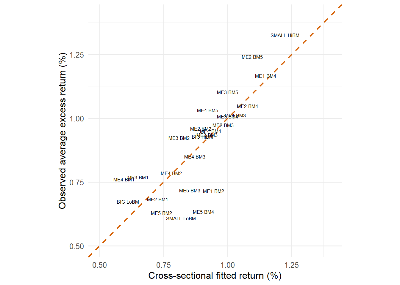
Figure 4.29: Cross-sectional fitted returns using estimated betas.
The fitted-return figure is the visual version of the second-pass regression. Each label is one portfolio. Points close to the 45-degree line are portfolios whose average returns are close to what the estimated beta prices predict. Points above the line have observed average returns larger than the fitted value; points below the line have observed average returns smaller than the fitted value.
Code
cross_section_aug |>select(symbol, ERe_percent, fitted_return_percent = .fitted) |>arrange(symbol) |>mutate(across(where(is.numeric), ~round(.x, 4))) |>kable(caption ="Observed and fitted average excess returns from the beta method.",row.names =FALSE ) |>kable_styling(latex_options ="HOLD_position")
Observed and fitted average excess returns from the beta method.
symbol
ERe_percent
fitted_return_percent
BIG HiBM
0.9289
0.9012
BIG LoBM
0.6733
0.6102
ME1 BM2
0.7150
0.9455
ME1 BM3
1.0120
1.0306
ME1 BM4
1.1674
1.1483
ME2 BM1
0.6830
0.7269
ME2 BM2
0.9597
0.8947
ME2 BM3
0.9735
0.9821
ME2 BM4
1.0482
1.0778
ME2 BM5
1.2414
1.0959
ME3 BM1
0.7691
0.6497
ME3 BM2
0.9239
0.8102
ME3 BM3
0.9351
0.9196
ME3 BM4
1.0079
1.0000
ME3 BM5
1.1023
1.0002
ME4 BM1
0.7602
0.5946
ME4 BM2
0.7856
0.7794
ME4 BM3
0.8506
0.8721
ME4 BM4
0.9506
0.9332
ME4 BM5
1.0322
0.9223
ME5 BM2
0.6291
0.7415
ME5 BM3
0.7176
0.8520
ME5 BM4
0.6341
0.9060
SMALL HiBM
1.3264
1.2245
SMALL LoBM
0.6080
0.8166
The fitted-value table gives the same comparison portfolio by portfolio. It is useful when labels overlap in the figure or when the reader wants to inspect a particular size-value cell directly.
The coefficients \(\lambda_M\), \(\lambda_S\), and \(\lambda_H\) are estimated prices of risk. A positive \(\lambda_H\), for example, means that portfolios with higher value exposure have higher average excess returns in this cross-section, conditional on the other beta estimates.
The fitted-return graph and fitted-value table should be read together. The graph shows the overall geometry: points close to the 45-degree line are well-explained by the beta-pricing equation. The table makes the individual portfolio comparison auditable. Large vertical gaps indicate portfolios whose average returns remain far from the fitted values implied by the estimated prices of market, size, and value exposure.
The reason for doing this second pass is conceptual. A time-series regression gives each portfolio’s market beta, size beta, and value beta. The next question is whether those betas carry enough information to account for the portfolio’s average return. The second pass asks that question directly. It treats the estimated betas as the characteristics to be priced and asks whether a common set of lambdas can assign reasonable average returns to all 25 portfolios at once.
The equation also clarifies the division of responsibility between data, estimation, and interpretation:
This table is also a guide to the code. cross_section_data contains the first two rows of the table: average excess returns and estimated betas. cross_section_fit estimates the lambdas. cross_section_aug adds fitted values and pricing errors. The code therefore follows the same sequence as the econometric argument: construct the cross-section, estimate prices of risk, then inspect the errors.
4.9 SDF-GMM and pricing logic
The beta-method prices exposures. The SDF-GMM method prices payoffs through moments. Both approaches ask whether the factor model can explain average excess returns, but they organize the evidence differently. The beta-method starts with estimated betas. SDF-GMM starts with a pricing condition and turns that condition into sample moments.
The purpose of this section is to make Cochrane’s chapter 13 operational. The logic is:
Step
Question
Object
Pricing condition
What should be true if the model prices excess returns?
\(E(m_tR_{i,t}^e)=0\)
Linear SDF
How does the discount factor depend on factors?
\(m_t=1-\mathbf{b}^{\top}\mathbf{f}_t\)
Sample moments
What does the model leave unexplained in the data?
What SDF loadings minimize unweighted pricing errors?
\(W=I\)
Second-stage GMM
What changes when errors are weighted by their covariance?
\(W=\widehat{\mathbf{S}}^{-1}\)
J-test
Are the remaining pricing errors jointly large?
\(J=T\mathbf{g}'W\mathbf{g}\)
This sequence answers a question beyond the regression table: after choosing the SDF loadings, are the leftover pricing errors small enough to be consistent with the model?
The stochastic discount factor view starts from the pricing condition
\[
E(m_t R_{i,t}^e)=0.
\]
This notation is standard in modern asset pricing (Cochrane 2005). The object \(m_t\) is a stochastic discount factor. It assigns value today to future payoffs. For an excess return, the initial cost is zero after financing at the risk-free rate. The model therefore asks for the discounted excess return to average to zero. The equation says that, after the model applies its discount factor, each test asset should have zero remaining average payoff.
Read the equation literally from inside to outside. Start with the excess return of asset \(i\) in month \(t\), \(R_{i,t}^e\). Multiply that payoff by the discount factor in the same month, \(m_t\). Then take the average implied by \(E(\cdot)\). If the model prices the asset, that average is zero because an excess return has zero initial cost. In the data, the sample version of this average is the pricing error. A model with small pricing errors is a model whose discount factor makes the test assets close to zero-cost payoffs in present-value terms.
The equation can be read in three layers. First, \(R_{i,t}^e\) is the payoff to be priced. Second, \(m_t\) is the risk adjustment applied to that payoff. Third, the expectation averages the risk-adjusted payoff over time or across states. If the model is correct, positive and negative risk-adjusted payoffs balance out for every test asset. The empirical version checks whether that balance is close enough in the sample.
The condition is easier to read through states of the world. If \(m_t\) is high in bad states, then payoffs received in those states are especially valuable. An asset that performs poorly when \(m_t\) is high must compensate investors with a higher average excess return. This is the same economic idea behind factor betas, written in pricing-condition form.
The condition also explains why covariance is central. The expectation \(E(m_tR_{i,t}^e)\) is an average product. It is affected by the average excess return of the asset and by the way that return co-moves with the discount factor. A high average excess return can be consistent with the model when the asset pays off in states where the discount factor is low. The asset is then less valuable as insurance, so investors require compensation through a higher average return.
A linear SDF can be normalized as
\[
m_t
=
1
-
\mathbf{b}^{\top}\mathbf{f}_t.
\]
This is the normalization used for the GMM calculation below. The constant is fixed at one, and the vector \(\mathbf{b}\) controls how strongly each factor enters the discount factor. If a factor captures bad times for investors, assets that pay poorly when that factor is adverse should require higher average excess returns. The SDF formulation and the beta-pricing formulation organize the same economic idea: systematic covariance with factors drives average returns.
The minus sign is useful for interpretation. With \(m_t=1-\mathbf{b}^{\top}\mathbf{f}_t\), a positive loading \(b_j\) means that months with a high value of factor \(f_j\) reduce the discount factor. In the expected-return equation below, that same positive \(b_j\) gives a positive contribution to a portfolio whose return has a positive sample moment with \(f_j\). The loading is therefore read as the price attached to that return-factor moment.
Substituting the linear SDF into the pricing condition gives the bridge from the theory to the data:
This last equation is the key pedagogical bridge. The average excess return is linked to moments of the form \(E(f_{j,t}R_{i,t}^e)\). The code below constructs sample versions of those moments for every portfolio and every factor. The estimated cross-sectional regression then asks whether those moments explain the same average excess returns studied in the beta method.
For the full cross-section of \(N\) test assets, define
This notation is compact, so it is worth mapping it to the objects used in the code:
Mathematical object
Code object
Interpretation
\(\bar{\mathbf{R}}^e\)
mean_returns
The vector of average excess returns for the 25 portfolios.
\(\mathbf{D}\)
moment_matrix
The matrix of return-factor sample moments.
\(\mathbf{b}\)
b1 or b2
The SDF loadings estimated by GMM.
\(\mathbf{D}\mathbf{b}\)
fitted_returns
The average excess returns implied by the SDF.
\(\mathbf{g}_T(\mathbf{b})\)
pricing_errors
Observed average returns minus fitted average returns.
\(\widehat{\mathbf{S}}_1\)
moment_covariance
The covariance matrix of the pricing-moment time series.
The dimensions also help. In the FF3 case there are \(N=25\) test portfolios and \(K=3\) factors. Therefore \(\bar{\mathbf{R}}^e\) has 25 entries, \(\mathbf{D}\) has 25 rows and 3 columns, \(\mathbf{b}\) has 3 entries, and \(\mathbf{g}_T(\mathbf{b})\) has 25 pricing errors. The model has fewer SDF loadings than portfolios, so it is overidentified. That is why the chapter can estimate the loadings and still test whether the remaining errors are too large.
The goal of SDF-GMM is to choose \(\mathbf{b}\) so these pricing errors are small. The first-stage and second-stage estimates differ in how they weight those errors.
The first-stage GMM estimate uses identity weighting, \(W=I\). Cochrane shows that, in this linear SDF setting, this estimate is an OLS cross-sectional regression of average returns on second moments (Cochrane 2005):
This equation is OLS without a cross-sectional intercept. The left-hand side is the vector of average excess returns. The regressors are the columns of \(\mathbf{D}\), the return-factor second moments. The estimated vector \(\widehat{\mathbf{b}}_1\) gives the SDF loadings that make \(\mathbf{D}\widehat{\mathbf{b}}_1\) as close as possible to \(\bar{\mathbf{R}}^e\) in ordinary least-squares distance.
The identity matrix is the natural first step because it requires only the average returns and the return-factor moments. It gives each portfolio’s pricing error equal weight in the criterion \(\mathbf{g}_T(\mathbf{b})^{\top}\mathbf{g}_T(\mathbf{b})\). This stage is the cleanest place to see the geometry of the SDF problem: choose the factor loadings that make the fitted vector \(\mathbf{D}\mathbf{b}\) close to the observed vector \(\bar{\mathbf{R}}^e\).
The empirical content comes from sample moments such as
The moment \(\widehat{E}(R_i^e f_j)\) is an average product. It is large when portfolio \(i\) tends to have high excess returns in months when factor \(j\) is high. It is negative when the portfolio tends to move against the factor. In applied work, these moments are useful because they turn co-movement into regressors that can be used in a cross-sectional pricing equation.
In matrix form, the code builds these quantities with
where \(\mathbf{R}\) is a \(T \times N\) matrix of portfolio excess returns and \(\mathbf{F}\) is a \(T \times K\) matrix of factor returns. The result \(\mathbf{D}\) is an \(N \times K\) matrix: one row for each test portfolio and one column for each factor moment.
The code below implements the FF3 first-stage GMM estimate. All estimation is done in decimal returns. Tables and figures convert average returns and pricing errors to percent for readability.
The first table is the cross-sectional dataset: one row per portfolio, return-factor second moments as regressors, observed average excess return as the target, and the resulting pricing error. The coefficient table reports the SDF loadings \(\widehat{\mathbf{b}}_1\). The summary table reports the identity-weighted GMM criterion and descriptive pricing-error measures. This is the exact first-stage object in Cochrane’s linear SDF-GMM setup: OLS cross-sectional fitting with \(W=I\).
The three tables should be read in order:
Table
How to read it
Why it is useful
First-stage data
Compare observed_percent, fitted_percent, and pricing_error_percent portfolio by portfolio.
It shows the actual cross-section being priced.
SDF loadings
Read the sign and size of each \(\widehat b_j\) relative to its standard error.
It shows which factor moments receive positive or negative prices.
Fit summary
Compare RMSE, MAE, maximum absolute error, and the identity criterion.
It summarizes the remaining pricing errors in a few auditable numbers.
The coefficient table is about the discount factor. The fit table is about the test assets. Keeping those two readings separate helps avoid a common confusion: a factor can have an economically meaningful SDF loading and the model can still leave sizable pricing errors for specific portfolios.
The second-stage estimate changes the weighting matrix. Define the moment vector for month \(t\) as
This covariance matrix measures how the pricing moments move together across months. If two portfolios are formed from nearby size-value cells, their pricing errors may be highly related. If one portfolio has especially volatile moment errors, its raw pricing error is less informative than a stable error of the same size. The second stage uses this information when it decides which errors should have more influence in the estimation criterion.
The second-stage estimate uses \(W=\widehat{\mathbf{S}}_1^{-1}\):
This is the GLS version of the same cross-sectional regression. Pricing errors with larger estimated covariance receive different weight from pricing errors with smaller estimated covariance. The point is efficiency: the second stage uses the covariance structure of the pricing moments, while the first stage weights all pricing errors equally.
The change from first stage to second stage has a specific interpretation. The target is still the same vector of average excess returns, and the regressors are still the same second moments. The weighting matrix changes the metric used to judge the errors. As a result, the second-stage fitted returns can move closer to some portfolios and farther from others. That movement is expected: the second-stage estimate tries to reduce the covariance-weighted error, so a smaller weighted criterion may occur even when the unweighted RMSE changes only slightly.
The first-stage and second-stage coefficient tables should be compared by factor. Large changes in \(\widehat{\mathbf{b}}\) indicate that the covariance weighting changes which pricing errors receive more influence in the estimation. The summary tables should be read together as well: the first-stage criterion reports the identity-weighted fit, and the second-stage criterion reports the covariance-weighted fit.
There are three useful reading questions at this point. First, do the signs of the SDF loadings remain stable across stages? Second, does covariance weighting materially change the size of the loadings? Third, do the pricing-error summaries improve in the metric that each stage is designed to minimize? These questions connect the algebra to interpretation: the second stage is a change in statistical weighting, so its economic meaning should be assessed through the fitted returns and the remaining pricing errors.
For FF3, the market loading remains positive across stages: 2.04 in the first stage and 1.91 in the second stage. The HML loading also remains positive, moving from 1.84 to 1.38. The size loading changes more, from -0.29 to 0.98. That movement tells the reader where covariance weighting has the largest effect: the statistical metric changes the role assigned to the size moment more than the role assigned to the market moment.
The overidentifying-restrictions test uses the pricing errors that remain after estimation:
\[
J
=
T
\mathbf{g}_T(\widehat{\mathbf{b}})^{\top}
\widehat{\mathbf{S}}_1^{+}
\mathbf{g}_T(\widehat{\mathbf{b}}),
\]
where \(\widehat{\mathbf{S}}_1^{+}\) is the generalized inverse of the first-stage moment covariance matrix. Under the usual large-sample GMM conditions, the statistic is compared with
\[
\chi^2_{N-K},
\]
where \(N\) is the number of test assets and \(K\) is the number of SDF factors. For FF3, \(N=25\) and \(K=3\), so the test has 22 degrees of freedom.
The J-test asks a joint question. After estimating \(K\) SDF loadings, are the \(N\) pricing conditions close enough to zero as a group? The degrees of freedom are \(N-K\) because the model uses \(K\) parameters to fit \(N\) moment conditions. A large p-value means the test provides little statistical evidence against the joint restrictions. A small p-value means the remaining pricing errors are too large relative to their covariance under the chi-square approximation. The test is statistical; the tables and figures that follow show the economic location and size of those errors.
The first-stage row reports two useful quantities. The identity criterion is the objective minimized by the first-stage OLS cross-sectional estimate. The J-statistic uses the estimated moment covariance matrix for the chi-square test. The second-stage row uses the same covariance weighting that defines the second-stage estimate. A small p-value indicates that the remaining pricing errors are large relative to their estimated covariance.
The distinction between the identity criterion and the J-statistic is important. The identity criterion is the fitting objective for the first-stage estimate. The J-statistic is the formal overidentifying-restrictions test, computed with the covariance weighting. Reporting both makes the calculation transparent: one number shows the first-stage distance that was minimized, and the other number gives the chi-square test of the pricing restrictions.
The first-stage SDF-GMM fitted-return figure should be compared with the beta-method fitted figure. Both plots use the same vertical axis, observed average excess return. The horizontal axis changes: the beta method uses fitted returns from estimated betas, while first-stage SDF-GMM uses fitted returns from return-factor second moments.
The reading rule is simple. A point on the dashed line means the model-implied average return equals the observed average return for that portfolio. A point above the line means the observed average return is higher than the fitted return, so the pricing error is positive. A point below the line means the model assigns too much average return to that portfolio. Labels far from the line are the portfolios that should be inspected in the fitted-value table.
Code
sdf_aug |>select(symbol, ERe_percent, fitted_return_percent = .fitted) |>arrange(symbol) |>mutate(across(where(is.numeric), ~round(.x, 4))) |>kable(caption ="Observed and fitted average excess returns from first-stage SDF-GMM.",row.names =FALSE ) |>kable_styling(latex_options ="HOLD_position")
Observed and fitted average excess returns from first-stage SDF-GMM.
symbol
ERe_percent
fitted_return_percent
BIG HiBM
0.9289
1.0953
BIG LoBM
0.6733
0.5881
ME1 BM2
0.7150
0.9593
ME1 BM3
1.0120
1.0094
ME1 BM4
1.1674
0.9645
ME2 BM1
0.6830
0.7814
ME2 BM2
0.9597
0.8397
ME2 BM3
0.9735
0.8705
ME2 BM4
1.0482
0.9351
ME2 BM5
1.2414
1.1095
ME3 BM1
0.7691
0.7761
ME3 BM2
0.9239
0.7608
ME3 BM3
0.9351
0.8159
ME3 BM4
1.0079
0.9016
ME3 BM5
1.1023
1.0911
ME4 BM1
0.7602
0.6499
ME4 BM2
0.7856
0.7498
ME4 BM3
0.8506
0.8116
ME4 BM4
0.9506
0.9019
ME4 BM5
1.0322
1.1395
ME5 BM2
0.6291
0.6421
ME5 BM3
0.7176
0.7250
ME5 BM4
0.6341
0.8791
SMALL HiBM
1.3264
1.1018
SMALL LoBM
0.6080
1.1312
The fitted-value table makes the first-stage SDF-GMM comparison explicit for each portfolio. Together with the graph, it lets the reader see which portfolios are matched closely and which remain difficult for the identity-weighted specification.
The beta method and first-stage SDF-GMM use different regressors, but they are both asking a cross-sectional asset pricing question: can a small set of factor-related quantities explain the average excess returns of the test assets?
First-stage SDF-GMM uses products \(R_i^e f_j\) as regressors. Each regressor measures how a portfolio return co-moves with a factor in the sample. The fitted values answer the same practical question as the beta method: given the factor information, what average excess return does the model assign to each portfolio?
The same SDF-GMM machinery can be run quickly for the two comparison models in the roadmap. The FF3-plus-momentum model adds the momentum factor to the same sample. The FF5 model uses the five-factor data and therefore starts later.
FF3 remains the detailed benchmark because it is the clearest bridge from the beta-method to SDF-GMM. The momentum and FF5 specifications are used as comparisons. Their role is to show how the same GMM logic changes when the factor set changes. The comparison is useful, but it should be read with care: adding a factor changes the model, and the FF5 data also change the available sample window.
SDF-GMM tests across FF3, FF3 plus momentum, and FF5.
model
stage
months
n_assets
n_factors
df
identity_criterion
j_statistic
p_value
FF3
First-stage GMM (W = I)
1128
25
3
22
0.075147
80.60545
0.000000
FF3
Second-stage GMM (W = S^-1)
1128
25
3
22
0.097174
78.38851
0.000000
FF3 plus momentum
First-stage GMM (W = I)
1128
25
4
21
0.032272
45.65241
0.001421
FF3 plus momentum
Second-stage GMM (W = S^-1)
1128
25
4
21
0.409426
42.83898
0.003296
FF5
First-stage GMM (W = I)
690
25
5
20
0.015023
61.61246
0.000004
FF5
Second-stage GMM (W = S^-1)
690
25
5
20
0.051550
54.59986
0.000047
Code
sdf_gmm_coefficients <-bind_rows( sdf_ff3_first_stage$coefficient_table, sdf_ff3_second_stage$coefficient_table, sdf_ff4_first_stage$coefficient_table, sdf_ff4_second_stage$coefficient_table, sdf_ff5_first_stage$coefficient_table, sdf_ff5_second_stage$coefficient_table)sdf_gmm_coefficients |>mutate(across(where(is.numeric), ~round(.x, 6))) |>kable(caption ="SDF-GMM loadings across the benchmark and comparison models.",row.names =FALSE ) |>kable_styling(latex_options ="HOLD_position")
SDF-GMM loadings across the benchmark and comparison models.
model
stage
factor
estimate
std_error
t_statistic
FF3
First-stage GMM (W = I)
Mkt_RF
2.040156
0.633179
3.222085
FF3
First-stage GMM (W = I)
SMB3
-0.293621
0.946250
-0.310300
FF3
First-stage GMM (W = I)
HML
1.842783
0.839478
2.195152
FF3
Second-stage GMM (W = S^-1)
Mkt_RF
1.907719
0.608701
3.134084
FF3
Second-stage GMM (W = S^-1)
SMB3
0.981290
0.878460
1.117057
FF3
Second-stage GMM (W = S^-1)
HML
1.384296
0.818106
1.692073
FF3 plus momentum
First-stage GMM (W = I)
Mkt_RF
5.163040
1.571232
3.285982
FF3 plus momentum
First-stage GMM (W = I)
SMB3
0.656010
1.514500
0.433153
FF3 plus momentum
First-stage GMM (W = I)
HML
9.867654
3.567355
2.766098
FF3 plus momentum
First-stage GMM (W = I)
Mom
15.480929
6.869332
2.253630
FF3 plus momentum
Second-stage GMM (W = S^-1)
Mkt_RF
4.923346
0.870037
5.658776
FF3 plus momentum
Second-stage GMM (W = S^-1)
SMB3
0.996144
1.204634
0.826927
FF3 plus momentum
Second-stage GMM (W = S^-1)
HML
8.279121
1.669757
4.958278
FF3 plus momentum
Second-stage GMM (W = S^-1)
Mom
16.477463
2.653309
6.210157
FF5
First-stage GMM (W = I)
Mkt_RF
4.222723
1.233189
3.424230
FF5
First-stage GMM (W = I)
SMB5
4.975657
1.526267
3.260018
FF5
First-stage GMM (W = I)
HML
-2.128367
4.151163
-0.512716
FF5
First-stage GMM (W = I)
RMW
12.312729
3.929934
3.133063
FF5
First-stage GMM (W = I)
CMA
11.583374
8.206800
1.411436
FF5
Second-stage GMM (W = S^-1)
Mkt_RF
5.113191
1.155828
4.423834
FF5
Second-stage GMM (W = S^-1)
SMB5
4.848905
1.456827
3.328402
FF5
Second-stage GMM (W = S^-1)
HML
1.506782
3.684959
0.408901
FF5
Second-stage GMM (W = S^-1)
RMW
18.225587
3.257656
5.594693
FF5
Second-stage GMM (W = S^-1)
CMA
8.034860
7.261619
1.106483
The comparison table should be read by model and by stage. Moving from FF3 to FF3 plus momentum changes the factor set while keeping the same test assets and sample. Moving to FF5 changes both the factor set and the sample window. The J-test p-value is the formal overidentifying-restrictions evidence for each SDF specification. The coefficient table then shows which SDF loadings drive those results.
The numerical message is clear. For FF3, the second-stage J-statistic is 78.39 with 22 degrees of freedom and a p-value of <0.001. Adding momentum lowers the second-stage J-statistic to 42.84, with a p-value of 0.003. That improvement is economically useful, but the formal test still rejects the joint pricing restrictions. FF5 also rejects in its shorter sample, with a second-stage p-value of <0.001. The conclusion is that all three SDF specifications leave statistically meaningful joint pricing errors for the 25 size-value portfolios.
The purpose of the comparison is diagnostic. If a richer factor set reduces pricing errors and weakens the J-test evidence against the model, then the additional factors are helping with this cross-section. If the pricing errors remain large or the J-test p-value remains small, then the extra factors have limited explanatory power for these test assets in this sample. The coefficient table then helps identify whether the added factor receives a meaningful SDF loading or enters weakly.
Selected FF3 portfolio comparisons by pricing method.
symbol
method
observed_percent
fitted_percent
pricing_error_percent
BIG HiBM
Beta
0.9289
0.9012
0.0276
BIG HiBM
SDF 1
0.9289
1.0953
-0.1664
BIG HiBM
SDF 2
0.9289
1.0462
-0.1173
BIG LoBM
Beta
0.6733
0.6102
0.0630
BIG LoBM
SDF 1
0.6733
0.5881
0.0852
BIG LoBM
SDF 2
0.6733
0.5936
0.0797
ME1 BM2
Beta
0.7150
0.9455
-0.2305
ME1 BM2
SDF 1
0.7150
0.9593
-0.2442
ME1 BM2
SDF 2
0.7150
1.1353
-0.4203
ME1 BM3
Beta
1.0120
1.0306
-0.0186
ME1 BM3
SDF 1
1.0120
1.0094
0.0026
ME1 BM3
SDF 2
1.0120
1.1385
-0.1265
ME1 BM4
Beta
1.1674
1.1483
0.0191
ME1 BM4
SDF 1
1.1674
0.9645
0.2029
ME1 BM4
SDF 2
1.1674
1.0898
0.0776
ME5 BM2
Beta
0.6291
0.7415
-0.1124
ME5 BM2
SDF 1
0.6291
0.6421
-0.0131
ME5 BM2
SDF 2
0.6291
0.6300
-0.0009
ME5 BM3
Beta
0.7176
0.8520
-0.1343
ME5 BM3
SDF 1
0.7176
0.7250
-0.0074
ME5 BM3
SDF 2
0.7176
0.6940
0.0237
ME5 BM4
Beta
0.6341
0.9060
-0.2719
ME5 BM4
SDF 1
0.6341
0.8791
-0.2450
ME5 BM4
SDF 2
0.6341
0.8408
-0.2067
SMALL HiBM
Beta
1.3264
1.2245
0.1019
SMALL HiBM
SDF 1
1.3264
1.1018
0.2246
SMALL HiBM
SDF 2
1.3264
1.2186
0.1078
SMALL LoBM
Beta
0.6080
0.8166
-0.2086
SMALL LoBM
SDF 1
0.6080
1.1312
-0.5231
SMALL LoBM
SDF 2
0.6080
1.2939
-0.6858
The FF3 comparison keeps the beta-method in the chapter. It is the expected-return beta regression from Cochrane chapter 12. First-stage SDF-GMM is the identity-weighted moment regression from Cochrane chapter 13. Second-stage SDF-GMM is the covariance-weighted version. The error-summary table shows which method leaves smaller pricing errors by RMSE, MAE, and maximum absolute error. The selected-portfolio table makes the comparison auditable at the portfolio level.
For these FF3 estimates, the beta-method has the lowest RMSE: 0.1138 percent per month. First-stage SDF-GMM has RMSE 0.1632, and second-stage SDF-GMM has RMSE 0.1856. The MAE comparison is closer, but the same table shows that the SDF versions produce larger maximum absolute errors in this sample. The empirical lesson is therefore specific: the SDF-GMM framework gives the formal moment test and the Cochrane-style weighting logic, while the static beta-method gives the smaller unweighted fitted-return errors for the FF3 cross-section used here.
Figure 4.31: Observed and fitted average excess returns across FF3 pricing methods.
The panel comparison gives the cleanest visual summary of the three methods. Each panel uses the same axes. Points closer to the 45-degree line are better priced by that method. Differences across panels show how the fitted cross-section changes when the model moves from beta pricing to first-stage and second-stage SDF-GMM.
The panels should be read as a model comparison with a common scale. A method that compresses points away from the 45-degree line underfits the dispersion in average returns. A method that places many points above or below the line in a similar direction leaves a systematic bias. A method with a few isolated large gaps may be capturing the broad pattern while struggling with particular size-value cells.
Figure 4.32: Pricing errors by portfolio across FF3 pricing methods.
The pricing-error plot reads the same information from a different angle. The zero line is perfect pricing. Points far from zero identify portfolios that remain difficult for a method. The grouped dots also show whether first-stage and second-stage SDF-GMM move errors in the same direction or change the portfolio-level pattern.
This plot is especially useful after the fitted-return panels. The fitted panels show distance from the 45-degree line. The error plot turns that distance into signed errors. Positive errors mean observed returns exceed fitted returns; negative errors mean fitted returns exceed observed returns. Reading the signs portfolio by portfolio helps identify whether a method consistently underprices or overprices particular size-value groups.
4.10 Pricing errors by size and value
A factor model can fit the cross-section well on average and still leave a visible pattern in the errors. Cochrane emphasizes this diagnostic in tests of characteristics: after a model is estimated, the remaining pricing errors should be inspected against the characteristics used to form the test assets (Cochrane 2005). In this chapter the relevant characteristics are size and book-to-market.
A positive value means that the portfolio earned more than the fitted value assigned by the model. A negative value means that the fitted value was higher than the observed average return. If the positive and negative errors cluster by size or value, the model still leaves a characteristic pattern unexplained.
This diagnostic connects the regression evidence back to the portfolio construction. The 25 portfolios were formed by sorting stocks into size and book-to-market cells. Those characteristics are visible in the labels before any model is estimated. A successful factor model should reduce the return pattern associated with those labels. After estimation, the heatmap asks a simple question: do the remaining errors still line up with the original size-value grid?
The answer guides interpretation. A few large errors scattered across the grid suggest asset-specific problems or noisy estimates. A block of errors in one row or one column suggests that the model has left a size or value pattern unexplained. This is why the diagnostic is more informative than a single goodness-of-fit number: it shows the location of the model’s failures.
The table identifies the portfolios where each method has the largest absolute pricing errors. It is a targeted audit: these are the cells that deserve attention before saying that a model explains the 25-portfolio cross-section.
Figure 4.33: Pricing errors across the size-value grid.
The heatmap makes the characteristic diagnostic visible. A random-looking mix of small positive and negative errors would be favorable for the model. Blocks of similar color along the size or value dimension indicate that the model is still missing a systematic pattern associated with the portfolio construction. This diagnostic is useful because the 25 portfolios were formed precisely to make those characteristic patterns visible.
Read one heatmap cell as follows. The row gives the size group, the column gives the book-to-market group, and the number inside the cell gives the pricing error in monthly percent units. Orange cells have observed average returns above the fitted value. Blue cells have fitted values above observed average returns. A useful model should make the heatmap visually quiet: small numbers, weak color, and absence of a clear row or column pattern. A model that leaves a strong color block is telling the reader where its factor structure is incomplete for this cross-section.
4.11 Implementation checks and econometric limits
The main implementation risk in factor models is losing the connection between units, equations, and samples. These checks keep the workflow auditable:
Check
Why it is important
Decimal returns in estimation
Regression coefficients assume returns and factors are in the same units.
Month-end dates
Asset returns and factors must align on the same calendar month.
Excess returns
Test-asset returns must subtract the risk-free rate before estimation.
Sample windows
FF3, momentum, and FF5 have different starting dates.
Intercepts
Alphas are pricing errors after controlling for the chosen factors.
Betas
Betas are exposures estimated from time-series regressions.
Cross-section
The second-pass regression tests whether estimated exposures explain average returns.
Pricing errors
Remaining errors should be read against the characteristics used to form the portfolios.
The chapter deliberately keeps the code close to the equations. The data download creates factor and portfolio returns. The time-series regressions estimate \(\alpha_i\) and \(\boldsymbol{\beta}_i\). The fitted expected-return equation converts those estimates into model-implied average excess returns. The cross-sectional beta regression tests whether factor exposures explain the 25 portfolio averages. The SDF-GMM blocks test whether return-factor moments price the same portfolios under first-stage and second-stage weighting. The final characteristic diagnostic asks where the remaining errors are located.
The sequence can be read as a translation table from Cochrane-style notation to applied work in R:
Econometric idea
Question in words
Where the chapter answers it
Factor exposure
How sensitive is each test asset to common risk factors?
Time-series regressions and beta tables.
Expected-return pricing
Do those exposures explain average returns across assets?
Cross-sectional beta-method regression.
SDF moment condition
Can one discount factor make all excess returns average to zero?
First-stage and second-stage SDF-GMM.
Overidentification
Are the remaining moment errors statistically too large?
J-test tables.
Economic diagnosis
Which portfolios remain hard to price, and why might that pattern be meaningful?
Fitted-return plots, error tables, and size-value heatmaps.
This translation is the main reason for writing the chapter in this style. A reader should be able to move from an equation to a code object, from the code object to a table or figure, and from the table or figure to an economic interpretation.
The same workflow has important econometric limits:
Limit
Consequence for interpretation
Static two-pass regression
The chapter estimates one cross-section of average returns. A formal Fama-MacBeth analysis would estimate prices of risk period by period.
Estimated betas
The second-pass regressors are generated from first-pass regressions. Formal inference would account for that extra uncertainty.
Alpha inference
The chapter reads alphas economically and diagnostically. A formal joint test of alphas, such as a GRS-style test, is a natural extension.
SDF-GMM weighting
The chapter implements first-stage identity weighting and second-stage covariance weighting with a zero-lag moment covariance matrix. HAC or iterated GMM would be natural extensions.
J-test
The J-test is reported for the SDF-GMM moments. Its interpretation relies on the large-sample chi-square approximation.
Standard errors
The displayed OLS and GMM tables are useful for orientation. Strong inference in financial returns often requires heteroskedasticity and autocorrelation corrections.
Data source
Downloaded financial data can change because of vendor corrections, ticker history, or file updates. The fixed sample end makes the exercise easier to audit.
These limits define the chapter’s scope: build the bridge from factor-model equations to R code, fitted returns, pricing errors, and economic interpretation.
4.12 Conclusion
This chapter extends the book from forecasting and volatility into asset pricing econometrics. The object of interest is an estimated relation between average excess returns and systematic risk exposures.
The empirical logic has five layers. First, factor returns define candidate sources of systematic risk. Second, time-series regressions estimate each asset’s exposure to those factors. Third, cross-sectional regressions evaluate whether those exposures explain average returns across test assets. Fourth, SDF-GMM writes the same pricing problem as moment restrictions, estimates first-stage and second-stage SDF loadings, and tests overidentifying restrictions. Fifth, pricing-error diagnostics show where the model still leaves structure in the size-value grid.
The Fama-French chapter also illustrates a broader lesson for applied financial econometrics: a model is useful only when the equation, data construction, estimation code, and economic interpretation remain connected.
Carhart, Mark M. 1997. “On Persistence in Mutual Fund Performance.”The Journal of Finance 52 (1): 57–82.
Cochrane, John H. 2005. Asset Pricing. Revised. Princeton University Press.
Fama, Eugene F., and Kenneth R. French. 1992. “The Cross-Section of Expected Stock Returns.”The Journal of Finance 47 (2): 427–65.
Fama, Eugene F., and Kenneth R. French. 1993. “Common Risk Factors in the Returns on Stocks and Bonds.”Journal of Financial Economics 33 (1): 3–56.
Fama, Eugene F., and Kenneth R. French. 2015. “A Five-Factor Asset Pricing Model.”Journal of Financial Economics 116 (1): 1–22.
Fama, Eugene F., and James D. MacBeth. 1973. “Risk, Return, and Equilibrium: Empirical Tests.”Journal of Political Economy 81 (3): 607–36.
Lintner, John. 1965. “The Valuation of Risk Assets and the Selection of Risky Investments in Stock Portfolios and Capital Budgets.”The Review of Economics and Statistics 47 (1): 13–37.
Mossin, Jan. 1966. “Equilibrium in a Capital Asset Market.”Econometrica 34 (4): 768–83.
Sharpe, William F. 1964. “Capital Asset Prices: A Theory of Market Equilibrium Under Conditions of Risk.”The Journal of Finance 19 (3): 425–42.