1 Logistic credit scoring
A lender receives loan applications before it knows which borrowers will repay and which borrowers will default. The practical problem is to use the information available at origination, such as income, loan amount, interest rate, age, credit grade, employment history, and other borrower characteristics, to estimate a probability of default for each applicant. That probability is useful only if it can be translated into a decision. Should the applicant be accepted or rejected? How many defaults will the bank accept if it approves 80% of applications? What happens if it becomes more selective and approves only 65%? This chapter follows that decision path from data to model, from model to predicted probability, from predicted probability to cutoff rule, and from cutoff rule to credit policy.
Two current examples motivate the workflow. Banca d’Italia’s in-house credit assessment system produces one-year PDs every month for hundreds of thousands of non-financial firms and keeps the statistical model readable by relying on logit regression, with selected machine-learning components for nonlinear patterns (Narizzano et al. 2024). In consumer credit, the CFPB emphasizes that lenders using conventional models or complex algorithms must provide accurate and specific reasons when an application is denied or otherwise receives adverse action (Consumer Financial Protection Bureau 2022). These examples explain why this chapter treats interpretation, validation, and cutoff decisions as part of credit modeling itself.
The chapter develops the workflow from loan-level data exploration to model estimation, evaluation, and credit policy decisions. This first part is informed by Hull’s credit risk chapters and by Lore Dirick’s DataCamp course materials on credit risk modeling in R, and it expands the discussion with more explicit links between model assumptions, R objects, diagnostic plots, classification rules, and bank strategy.
1.1 The credit scoring problem
The practical credit-scoring problem begins before the bank knows the outcome of a loan. At origination, the bank observes borrower and loan characteristics, such as age, income, loan amount, interest rate, grade, and employment history. The repayment outcome is still unknown. The model’s job is to turn the information available at origination into a probability of default that can support a lending decision.
This is a binary prediction problem because each historical loan has one of two observed outcomes, default or no default. In this chapter, logistic regression gives us a transparent first benchmark. We estimate the model on a training sample, use it to generate predicted probabilities for new applicants in a test sample, and then ask whether those probabilities lead to useful credit decisions. The key object is a decision rule built from statistical predictions. It tells us which applications should be accepted, which should be rejected, and what bad rate follows from that rule.
We first load the required R packages.
1.2 Data exploration and cleaning
We begin by loading loan_data_ARF.rds and inspecting its structure before any modeling decisions are made. This database is available here.
'data.frame':   29092 obs. of  10 variables:
 $ loan_status   : int  0 0 0 0 0 0 1 0 1 0 ...
 $ loan_amnt     : int  5000 2400 10000 5000 3000 12000 9000 3000 10000 1000 ...
 $ int_rate      : num  10.6 11 13.5 11 11 ...
 $ grade         : Factor w/ 7 levels "A","B","C","D",..: 2 3 3 1 5 2 3 2 2 4 ...
 $ emp_length    : int  10 25 13 3 9 11 0 3 3 0 ...
 $ home_ownership: Factor w/ 4 levels "MORTGAGE","OTHER",..: 4 4 4 4 4 3 4 4 4 4 ...
 $ annual_inc    : num  24000 12252 49200 36000 48000 ...
 $ age           : int  33 31 24 39 24 28 22 22 28 22 ...
 $ sex           : Factor w/ 2 levels "0","1": 1 1 1 1 2 2 2 2 1 2 ...
 $ region        : Factor w/ 4 levels "E","N","S","W": 1 1 3 3 2 2 2 2 4 1 ...
This dataset represents the type of loan-level information a financial institution could use before making or reviewing a credit decision. It contains 29,092 observations across 10 variables. Each observation corresponds to the personal and loan characteristics of an individual loan.
The dependent variable is loan_st, which indicates loan status. A value of 0 represents no default, while a value of 1 represents default. A default occurs when a borrower fails to make timely payments, misses payments, or ceases payments on the interest or principal owed. The definition of default can vary depending on the goals and interests of the analysis. For the purposes of this study, we classify loans simply as either default or no default.
The variable loan_st is dichotomous, or categorical. Our primary interest lies in predicting whether a new loan application will result in default or not.
loan_data_ARF.rds contains historical information because the repayment outcome is already known. Historical data is valuable for understanding how borrower and loan characteristics relate to default. It is also the basis for training quantitative models and evaluating how those models behave on new applicants.
Several variable names can be shortened without losing their meaning. We rename them before continuing.
Code
| Original.name | Book.name |
|---|---|
| loan_status | loan_st |
| loan_amnt | l_amnt |
| int_rate | int |
| grade | grade |
| emp_length | emp_len |
| home_ownership | home |
| annual_inc | income |
| age | age |
| sex | sex |
| region | region |
The dataset now has shorter variable names.
The first 10 rows give a quick view of the variables and their coding.
Code
| loan_st | l_amnt | int | grade | emp_len | home | income | age | sex | region |
|---|---|---|---|---|---|---|---|---|---|
| 0 | 5000 | 10.65 | B | 10 | RENT | 24000 | 33 | 0 | E |
| 0 | 2400 | 10.99 | C | 25 | RENT | 12252 | 31 | 0 | E |
| 0 | 10000 | 13.49 | C | 13 | RENT | 49200 | 24 | 0 | S |
| 0 | 5000 | 10.99 | A | 3 | RENT | 36000 | 39 | 0 | S |
| 0 | 3000 | 10.99 | E | 9 | RENT | 48000 | 24 | 1 | N |
| 0 | 12000 | 12.69 | B | 11 | OWN | 75000 | 28 | 1 | N |
| 1 | 9000 | 13.49 | C | 0 | RENT | 30000 | 22 | 1 | N |
| 0 | 3000 | 9.91 | B | 3 | RENT | 15000 | 22 | 1 | N |
| 1 | 10000 | 10.65 | B | 3 | RENT | 100000 | 28 | 0 | W |
| 0 | 1000 | 16.29 | D | 0 | RENT | 28000 | 22 | 1 | E |
Note that sex is 1 for female and 0 for male. A categorical variable such as home can be summarized with the CrossTable() function.
   Cell Contents
|-------------------------|
|                       N |
|         N / Table Total |
|-------------------------|


Total Observations in Table:  29092


          |  MORTGAGE |     OTHER |       OWN |      RENT |
          |-----------|-----------|-----------|-----------|
          |     12002 |        97 |      2301 |     14692 |
          |     0.413 |     0.003 |     0.079 |     0.505 |
          |-----------|-----------|-----------|-----------|
CrossTable() can also summarize two variables at once. Adding loan_st to the home-ownership table lets us compare default behavior across home-ownership categories.
Code
   Cell Contents
|-------------------------|
|                       N |
|           N / Row Total |
|-------------------------|


Total Observations in Table:  29092


             | dat$loan_st
    dat$home |         0 |         1 | Row Total |
-------------|-----------|-----------|-----------|
    MORTGAGE |     10821 |      1181 |     12002 |
             |     0.902 |     0.098 |     0.413 |
-------------|-----------|-----------|-----------|
       OTHER |        80 |        17 |        97 |
             |     0.825 |     0.175 |     0.003 |
-------------|-----------|-----------|-----------|
         OWN |      2049 |       252 |      2301 |
             |     0.890 |     0.110 |     0.079 |
-------------|-----------|-----------|-----------|
        RENT |     12915 |      1777 |     14692 |
             |     0.879 |     0.121 |     0.505 |
-------------|-----------|-----------|-----------|
Column Total |     25865 |      3227 |     29092 |
-------------|-----------|-----------|-----------|
Code
home_default_summary <- dat |>
  mutate(default = as.numeric(as.character(loan_st))) |>
  group_by(home) |>
  summarize(
    loans = n(),
    defaults = sum(default == 1),
    default_rate = mean(default == 1),
    .groups = "drop"
  )

home_default_summary |>
  mutate(default_rate = fmt_pct(default_rate, 2)) |>
  knitr::kable(
    caption = "Default rate by home-ownership category.",
    row.names = FALSE
)| home | loans | defaults | default_rate |
|---|---|---|---|
| MORTGAGE | 12002 | 1181 | 9.84% |
| OTHER | 97 | 17 | 17.53% |
| OWN | 2301 | 252 | 10.95% |
| RENT | 14692 | 1777 | 12.10% |
The table reports defaults by home ownership. The row percentages in CrossTable() answer a credit-risk question. Conditional on belonging to a given home-ownership category, what fraction of loans defaulted? The compact table repeats the same idea as a default rate. For example, the mortgage row says that loans associated with borrowers in the mortgage category have a default rate of 9.84% in this sample. This is not yet a causal statement. It is a descriptive relationship that helps us see whether home ownership may contain useful information for credit scoring.
For numerical variables, plots are often easier to read than raw tables. The next figure shows the interest-rate distribution.
Code
interest_quantiles <- quantile(dat$int, probs = c(0.25, 0.5, 0.75), na.rm = TRUE)

ggplot(dat, aes(x = int)) +
  geom_histogram(aes(y=..density..), binwidth = 0.5, colour = "black",
                 fill = "white") +
  labs(y = "Density", x = "Interest rate") +
  theme(legend.position = "bottom", legend.title = element_blank())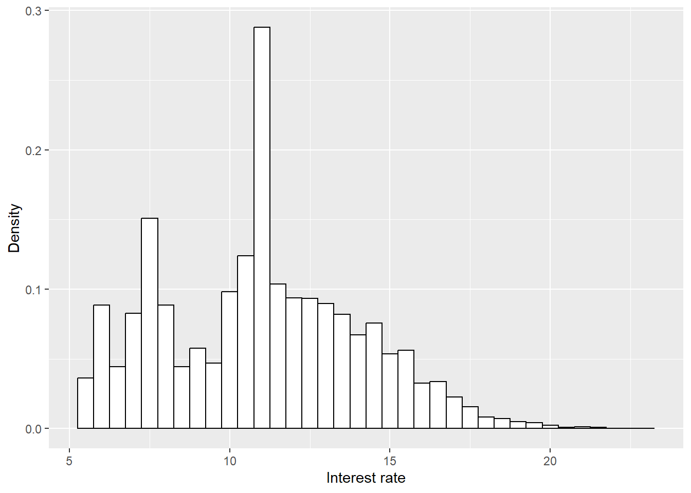
The histogram shows where the observed loan interest rates are concentrated before modeling. Most of the mass lies between the first and third quartiles, from 8.49 to 13.11, with a median of 10.99. This affects interpretation because the model will learn the relationship between interest rates and default mainly from the range where many loans are observed. Sparse tails should be read with more caution.
The next dotplot shows annual income.
Code
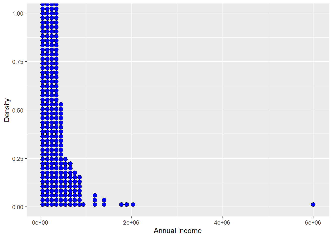
The Figure 1.2 above appears suspicious. The horizontal axis shows a very large annual income value (6e+06). Additionally, there are only a few individuals with extremely high incomes. We should investigate further to determine whether these observations should remain in the analysis or whether they distort the visual and statistical summary of the rest of the sample.
      loan_st l_amnt   int grade emp_len     home  income age sex region
4861        0  12025 14.27     C      13     RENT 1782000  63   0      E
13931       0  10000  6.54     A      16      OWN 1200000  36   0      W
15386       0   1500 10.99     A       5 MORTGAGE 1900000  60   1      N
16713       0  12000  7.51     A       1 MORTGAGE 1200000  32   0      E
19486       0   5000 12.73     C      12 MORTGAGE 6000000 144   1      E
22811       0  10000 10.99     A       1 MORTGAGE 1200000  40   1      E
23361       0   6400  7.40     A       7 MORTGAGE 1440000  44   1      E
23683       0   6600  7.74     A       9 MORTGAGE 1362000  47   0      E
28468       0   8450 12.29     C       0     RENT 2039784  42   0      E
One individual (ID 19486) combines an extremely high income with an age of 144. The age value is implausible, and the income values are extreme relative to the rest of the sample. In this book we continue with an analysis without these extreme observations. This is a discretionary cleaning criterion. In an applied project, we would document the decision and usually compare results with and without these observations.
The original dataset contains 29,092 rows. After removing 9 observations, the cleaned dataset contains 29,083 rows.
Code
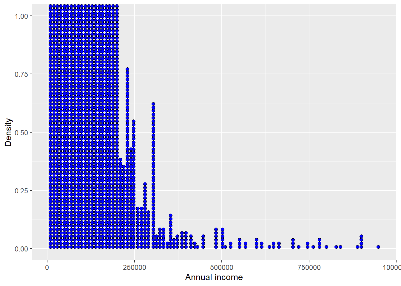
The revised plot is easier to read because the extreme observations no longer compress the main income distribution.
We also inspect summary statistics by sex.
Code
# A tibble: 2 × 7
  sex     Mean Median   Min    Max Count Gender
  <fct>  <dbl>  <dbl> <dbl>  <dbl> <int> <chr>
1 0     66021.  56000  4000 900000 13877 Male
2 1     67064.  57000  4200 948000 15206 Female
The table shows that, in this dataset, observations labeled as female have slightly higher average and median incomes compared to observations labeled as male. The income distribution for females also appears more variable, with a wider range of incomes. This summary must be interpreted carefully because the sex variable was added for teaching purposes and should not be treated as evidence about gender and income in a real population. In applied credit risk work, variables related to protected characteristics, and variables that may proxy for them, require explicit legal, ethical, and fairness review before they are used in modeling or decision rules.
The exploration above gives us enough context to proceed. Data cleaning can continue indefinitely, so an applied project has to balance inspection with the modeling objective. We have checked the outcome definition, simplified variable names, removed implausible extreme income observations, and reviewed a few basic summaries. The next section uses the cleaned data to estimate logistic credit-scoring models.
1.3 Logistic regression models
Logistic regression is the first credit-scoring model in the book because it is transparent and directly produces probabilities of default. The dependent variable is loan_st, where 1 means default and 0 means no default. The model output is not immediately a default/no-default label. Its first output is a probability between 0 and 1. A later cutoff rule converts that probability into a binary lending decision. A good reference for this section is Hull (2020).
We split the data into a training set and a test set. The training set is used to estimate the model. The test set is held back and used later to evaluate predictions on observations that were not used for estimation. The separation is essential because a model can fit historical defaults well and still perform poorly on new loan applications.
Code
# Set loan status as a factor.
dat$loan_st <- as.factor(dat$loan_st)
set.seed(567)
index_train <- cbind(runif(1 : nrow(dat), 0 , 1), c(1 : nrow(dat)))
index_train <- order(index_train[, 1])
index_train <- index_train[1: (2/3 * nrow(dat))]
# Create training set
train <- dat[index_train, ]
# Create test set
test <- dat[-index_train, ]
Factors are useful for categorical variables in R because they tell modeling and plotting functions that the variable takes a limited set of categories.
We have 29,083 observations in dat. The code above randomly selects 19,388 rows to form train. test contains the remaining 9,695 rows. Random selection helps avoid a split that accidentally reflects some ordering in the data. For example, if the first observations were mostly no-default loans, a non-random split could distort both estimation and evaluation.
The next table checks whether train and test preserve the basic default proportions in dat.
Code
# Combine data into a list for processing
data_list <- list(dat = dat$loan_st, train = train$loan_st, test = test$loan_st)

# Compute proportions and combine into a data frame
prop <- do.call(rbind, lapply(data_list, function(x) prop.table(table(x))))
colnames(prop) <- c("no defaults", "defaults")
row.names(prop) <- c("dat_prop", "train_prop", "test_prop")
prop
no defaults defaults
dat_prop 0.8890417 0.1109583
train_prop 0.8882298 0.1117702
test_prop 0.8906653 0.1093347The proportions of “defaults” and “no defaults” in the train and test datasets are very similar to those in the original dataset, indicating that both samples are representative. Specifically, the proportion of “defaults” in the train and test datasets closely matches that of the original dataset, as does the proportion of “no defaults.” This suggests that the random sampling process has preserved the overall distribution of the target variable, ensuring that the train and test sets reflect the characteristics of the full dataset.
This split is enough for the teaching objective of the chapter. It lets us estimate models on one sample and evaluate their behavior on observations that were held back from estimation. In a production workflow, however, we would usually add one more layer. Model choices such as variable selection, cutoffs, and tuning decisions should be made with a training/validation structure or cross-validation, while a final holdout test set should be reserved for the last evaluation. In this book we use the test set repeatedly to make the logic visible, so the results should be read as a controlled learning exercise with limited claims about production validation.
We begin with a deliberately simple and incomplete model that uses only age. This is a naive benchmark, not a serious final credit score. Its pedagogical role is to let us see the mechanics of logistic regression before adding predictors that are more closely tied to credit risk. To keep the mathematical notation separate from the code, let \(Y_i\) denote the value stored in loan_st for applicant \(i\), and let \(\text{age}_i\) denote that applicant’s age.
The model first defines the conditional probability that applicant \(i\) defaults:
\[ p_i = P(Y_i = 1 \mid \text{age}_i). \]
Then logistic regression assumes that the log-odds of that probability are linear in age:
\[ \log\left(\frac{p_i}{1-p_i}\right) = \beta_0 + \beta_1 \times \text{age}_i. \]
This equation intentionally omits an additive error term \(\varepsilon_i\). In a linear regression, the error term is added to the equation for the observed outcome. In logistic regression, the observed outcome is binary, so the randomness is described by \(Y_i \mid \text{age}_i \sim \text{Bernoulli}(p_i)\). The logit equation describes the conditional probability \(p_i\) that generates the realized 0/1 outcome.
Where:
\(Y_i\) is the observed outcome in the data: \(Y_i=1\) means default and \(Y_i=0\) means no default.
\(p_i\) is the probability that applicant \(i\) defaults, conditional on age.
\(\beta_0\) is the intercept, and \(\beta_1\) is the coefficient for the predictor variable
age.
The dependent variable in logistic regression remains binary. In the data, loan_st is either 0 or 1. The model transforms the conditional probability of default, \(p_i\), which generates the observed 0/1 outcome. The transformation \(\log\left(\frac{p_i}{1-p_i}\right)\), known as the logit function, maps probabilities \(p_i\), which range between 0 and 1, to the entire real number line \(-\infty\) to \(+\infty\). This allows the model to establish a linear relationship between the independent variable(s), such as age, and the transformed probability. The fraction \(\frac{p_i}{1-p_i}\), called the odds, represents the ratio of the probability of an event happening \(p_i\) to the probability of it not happening \(1-p_i\), making it a natural choice for modeling binary outcomes.
We estimate the age model with glm().
Code
Call:  glm(formula = loan_st ~ age, family = "binomial", data = train)

Coefficients:
(Intercept)          age
   -1.90097     -0.00623

Degrees of Freedom: 19387 Total (i.e. Null);  19386 Residual
Null Deviance:      13580
Residual Deviance: 13580    AIC: 13580
The equation and the code correspond directly. In glm(loan_st ~ age, family = "binomial", data = train), the left side of ~ is the observed \(Y_i\), the right side is the predictor \(\text{age}_i\), and family = "binomial" tells R to estimate the logit model. The coefficients \(\beta_0\) and \(\beta_1\) are the numbers returned by glm(), and later predict(logi_age, newdata = ..., type = "response") will transform the logit score back into the estimated probability \(\hat p_i\).
The estimated model is \(\log\left(\frac{p_i}{1-p_i}\right) = -1.90097 - 0.00623 \times \text{age}_i\).
The model suggests there is a negative relationship between age and loan status.
Solving for \(p_i\) gives the estimated probability of default according to the age model. The expression is \(p_i = \frac{\exp(-1.90097 - 0.00623 \times \text{age}_i)}{1 + \exp(-1.90097 - 0.00623 \times \text{age}_i)}\). We now evaluate \(p_i\) at two ages.
For \(\text{age} = 18\), \(p = \frac{\exp(-1.90097 - 0.00623 \times 18)}{1 + \exp(-1.90097 - 0.00623 \times 18)}\),
\(p = \frac{\exp(-2.01310)}{1 + \exp(-2.01310)} = \frac{0.1336}{1 + 0.1336} = 0.1178 = 11.78%\).
For \(\text{age} = 60\), \(p = \frac{\exp(-1.90097 - 0.00623 \times 60)}{1 + \exp(-1.90097 - 0.00623 \times 60)}\),
\(p = \frac{\exp(-2.27474)}{1 + \exp(-2.27474)} = \frac{0.1028}{1 + 0.1028} = 0.0932 = 9.32%\).
The default probability estimates at ages 18 and 60 are very close. The model therefore generates little separation in predicted default risk, even when evaluated over a wide age range. This is an early warning that age alone is a weak predictor for this credit scoring problem.
The next figure shows the logistic regression model’s output. The training data contain ages from 20 to 94. The model maps those two endpoints to predicted default probabilities of 11.65% and 7.68%, respectively. The dotted indicators in the figure mark those two observed age limits and their corresponding probabilities.
Code
# Define the function for the logistic regression model
logistic_function <- function(age) {
  beta0 <- beta_age_0
  beta1 <- beta_age_1
  p <- exp(beta0 + beta1 * age) / (1 + exp(beta0 + beta1 * age))
  return(p)
}

# Generate a sequence of ages
ages <- seq(-1000, 500, by = 1)

# Apply the logistic function to each age
p_values <- sapply(ages, logistic_function)

age_indicator_data <- data.frame(
  age = c(age_min_train, age_max_train),
  p = c(age_pd_min_train, age_pd_max_train),
  label_x = c(age_min_train + 80, age_max_train + 240),
  label_y = c(
    min(age_pd_min_train + 0.08, 0.95),
    min(age_pd_max_train + 0.22, 0.95)
  ),
  label = c(
    paste0("min age = ", fmt_num(age_min_train, 0), "\np = ", fmt_pct(age_pd_min_train, 2)),
    paste0("max age = ", fmt_num(age_max_train, 0), "\np = ", fmt_pct(age_pd_max_train, 2))
  )
)

# Create the plot
library(ggplot2)
ggplot(data = data.frame(age = ages, p = p_values), aes(x = age, y = p)) +
  geom_line(color = "blue", linewidth = 2) +
  geom_segment(
    data = age_indicator_data,
    aes(x = age, xend = age, y = 0, yend = p),
    inherit.aes = FALSE,
    linetype = "dotted",
    linewidth = 0.9,
    color = "#C0392B"
  ) +
  geom_segment(
    data = age_indicator_data,
    aes(x = min(ages), xend = age, y = p, yend = p),
    inherit.aes = FALSE,
    linetype = "dotted",
    linewidth = 0.9,
    color = "#C0392B"
  ) +
  geom_segment(
    data = age_indicator_data,
    aes(x = age, xend = label_x, y = p, yend = label_y),
    inherit.aes = FALSE,
    linetype = "dotted",
    linewidth = 0.7,
    color = "#C0392B"
  ) +
  geom_point(
    data = age_indicator_data,
    aes(x = age, y = p),
    inherit.aes = FALSE,
    color = "#C0392B",
    size = 2.8
  ) +
  geom_label(
    data = age_indicator_data,
    aes(x = label_x, y = label_y, label = label),
    inherit.aes = FALSE,
    size = 3.2,
    fill = "white",
    color = "#7B241C",
    label.size = 0.2
  ) +
  labs(x = "Age", y = "Probability (p)") +
  theme_minimal()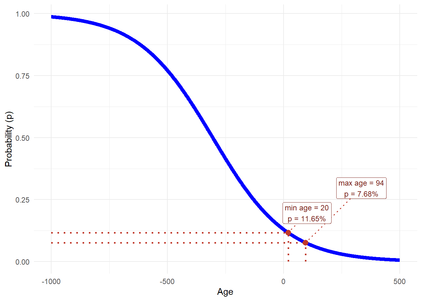
The logistic curve derived from this model is unreasonable because the probability \(p\) changes very slowly with respect to age. The dotted vertical lines show that the realistic age range in the training data is only a small segment of the very wide x-axis needed to display the full sigmoid curve. The dotted horizontal lines show the corresponding predicted probabilities, which move only from 7.68% to 11.65% across the observed age range, a difference of 3.97%. The age-only model therefore generates little meaningful separation in default probabilities for realistic applicants. To see probabilities close to 0 or 1, the model would require age values that are unrealistic or implausibly extreme.
The AIC value of the age model (13,581) is useful when comparing models estimated on the same response variable and sample. The Akaike information criterion (AIC) is a mathematical method for comparing in-sample fit while penalizing model complexity. In statistics, AIC is used to compare different possible models; lower AIC values indicate a better in-sample trade-off between fit and parsimony among the models being compared. At the moment we cannot interpret the AIC very much because we only have one model and we cannot compare it with another AIC.
The next candidate uses the interest rate as the only predictor of loan_st. At this stage we are still estimating models on the training set, before evaluating test-set predictions.
Code
Call:  glm(formula = loan_st ~ int, family = "binomial", data = train)

Coefficients:
(Intercept)          int
     -3.710        0.142

Degrees of Freedom: 19387 Total (i.e. Null);  19386 Residual
Null Deviance:      13580
Residual Deviance: 13210    AIC: 13220
The AIC is lower (13,216 versus 13,581), so this model has a better in-sample fit-parsimony trade-off than the age-only model.
Single-predictor models are useful for teaching, but they are too limited for a serious credit score. The logi_multi model adds age, interest rate, grade, loan amount, and annual income. We also use summary() to inspect more of the estimation output.
Code
Call:
glm(formula = loan_st ~ age + int + grade + log(l_amnt) + log(income),
    family = "binomial", data = train)

Coefficients:
             Estimate Std. Error z value Pr(>|z|)
(Intercept)  1.996240   0.477911   4.177 2.95e-05 ***
age         -0.002302   0.003825  -0.602   0.5473
int          0.038767   0.017249   2.247   0.0246 *
gradeB       0.503409   0.087435   5.758 8.54e-09 ***
gradeC       0.748229   0.117765   6.354 2.10e-10 ***
gradeD       0.964343   0.147283   6.548 5.85e-11 ***
gradeE       1.033442   0.190817   5.416 6.10e-08 ***
gradeF       1.619470   0.257900   6.279 3.40e-10 ***
gradeG       1.867494   0.440232   4.242 2.21e-05 ***
log(l_amnt)  0.015718   0.036341   0.433   0.6654
log(income) -0.470748   0.046423 -10.140  < 2e-16 ***
---
Signif. codes:  0 '***' 0.001 '**' 0.01 '*' 0.05 '.' 0.1 ' ' 1

(Dispersion parameter for binomial family taken to be 1)

    Null deviance: 13579  on 19387  degrees of freedom
Residual deviance: 13028  on 19377  degrees of freedom
AIC: 13050

Number of Fisher Scoring iterations: 5
The multi-factor model is a stronger candidate than the previous two. In logi_multi, the AIC value is the lowest so far (13,050 versus 13,216), so this should be considered the best in-sample model among these candidates at the moment. AIC is still an in-sample criterion. A lower AIC does not guarantee better predictive performance on new applications, so the model’s practical value must be checked later with the test set.
This is also the first output in the chapter where the full coefficient table is worth reading. The Estimate column reports effects on log-odds, not directly on probabilities. Std. Error measures estimation uncertainty. The z value divides the estimate by its standard error, and Pr(>|z|) is the p-value for testing whether the coefficient is zero after controlling for the other variables in the model. In credit terms, this asks whether the variable still contains information about default risk once age, interest rate, grade, loan amount, and income are considered together.
The log-odds scale is not intuitive, so the next table converts coefficients into odds ratios. If we exponentiate a coefficient with the exp() function, we obtain:
\[ \text{odds ratio}_j = \exp(\beta_j). \]
An odds ratio above 1 means higher odds of default, and an odds ratio below 1 means lower odds of default. The 95% interval helps us see whether the odds ratio is clearly different from 1. If the interval contains 1, the estimated direction is statistically unclear at the usual 5% level.
Code
multi_summary <- summary(logi_multi)$coefficients

odds_ratios <- data.frame(
  term = rownames(multi_summary),
  coefficient = multi_summary[, "Estimate"],
  std_error = multi_summary[, "Std. Error"],
  z_value = multi_summary[, "z value"],
  p_value = multi_summary[, "Pr(>|z|)"],
  OR = exp(multi_summary[, "Estimate"]),
  OR_low_95 = exp(multi_summary[, "Estimate"] - 1.96 * multi_summary[, "Std. Error"]),
  OR_high_95 = exp(multi_summary[, "Estimate"] + 1.96 * multi_summary[, "Std. Error"])
)
rownames(odds_ratios) <- odds_ratios$term

odds_ratios$reading <- ifelse(
  odds_ratios$p_value < 0.05 & odds_ratios$OR_low_95 > 1,
  "clear increase in odds",
  ifelse(
    odds_ratios$p_value < 0.05 & odds_ratios$OR_high_95 < 1,
    "clear decrease in odds",
    "unclear at 5%"
  )
)

grade_terms <- grep("^grade", rownames(odds_ratios), value = TRUE)
grade_significant_terms <- grade_terms[
  odds_ratios[grade_terms, "p_value"] < 0.05
]
grade_significant_labels <- sub("^grade", "", grade_significant_terms)
grade_reference <- if (is.factor(train$grade)) {
  levels(train$grade)[1]
} else {
  sort(unique(train$grade))[1]
}
grade_significant_text <- if (length(grade_significant_labels) > 0) {
  paste(grade_significant_labels, collapse = ", ")
} else {
  "none at this threshold"
}

grade_first_term <- if ("gradeB" %in% grade_terms) "gradeB" else grade_terms[1]
grade_first_label <- sub("^grade", "", grade_first_term)
grade_highest_term <- grade_terms[which.max(odds_ratios[grade_terms, "OR"])]
grade_highest_label <- sub("^grade", "", grade_highest_term)
grade_or_increases <- all(diff(odds_ratios[grade_terms, "OR"]) > 0)

odds_ratio_table <- odds_ratios[odds_ratios$term != "(Intercept)", ]
odds_ratio_table <- data.frame(
  Term = odds_ratio_table$term,
  Coefficient = fmt_num(odds_ratio_table$coefficient, 4),
  `Odds ratio` = fmt_num(odds_ratio_table$OR, 4),
  `95% OR interval` = paste0(
    "[",
    fmt_num(odds_ratio_table$OR_low_95, 4),
    ", ",
    fmt_num(odds_ratio_table$OR_high_95, 4),
    "]"
  ),
  `p-value` = format.pval(odds_ratio_table$p_value, digits = 3, eps = 0.001),
  Reading = odds_ratio_table$reading,
  check.names = FALSE
)

knitr::kable(
  odds_ratio_table,
  caption = "Coefficient and odds-ratio interpretation for `logi_multi`.",
  row.names = FALSE
)| Term | Coefficient | Odds ratio | 95% OR interval | p-value | Reading |
|---|---|---|---|---|---|
| age | -0.0023 | 0.9977 | [0.9902, 1.0052] | 0.5473 | unclear at 5% |
| int | 0.0388 | 1.0395 | [1.0050, 1.0753] | 0.0246 | clear increase in odds |
| gradeB | 0.5034 | 1.6544 | [1.3938, 1.9636] | <0.001 | clear increase in odds |
| gradeC | 0.7482 | 2.1133 | [1.6777, 2.6619] | <0.001 | clear increase in odds |
| gradeD | 0.9643 | 2.6231 | [1.9653, 3.5009] | <0.001 | clear increase in odds |
| gradeE | 1.0334 | 2.8107 | [1.9337, 4.0855] | <0.001 | clear increase in odds |
| gradeF | 1.6195 | 5.0504 | [3.0465, 8.3725] | <0.001 | clear increase in odds |
| gradeG | 1.8675 | 6.4721 | [2.7309, 15.3382] | <0.001 | clear increase in odds |
| log(l_amnt) | 0.0157 | 1.0158 | [0.9460, 1.0908] | 0.6654 | unclear at 5% |
| log(income) | -0.4707 | 0.6245 | [0.5702, 0.6840] | <0.001 | clear decrease in odds |
Now read the table as a credit model rather than as a list of statistics. The interest-rate coefficient is positive. Its odds ratio is 1.0395, so a one-unit increase in the recorded interest-rate variable multiplies the odds of default by 1.0395, holding age, grade, loan amount, and income fixed. Equivalently, the estimated odds are 3.95% higher. The p-value is 0.0246, so this association is statistically clear at the 5% level. In credit terms, loans with higher interest rates are associated with higher default risk after the other included variables are held fixed.
The grade coefficients give the clearest credit-risk pattern. R uses grade A as the reference category, so each grade coefficient compares that grade with grade A, holding the other variables fixed. In this estimation, 6 grade coefficients are statistically significant at the 5% level. They are B, C, D, E, F, G. The first reported grade comparison, grade B, has an odds ratio of 1.6544. The largest grade odds ratio is grade G, with 6.4721. The odds ratios rise as the grade worsens from B to G, which is exactly the pattern a credit analyst would expect from a risk grade.
Income moves in the opposite direction. The odds ratio for log(income) is 0.6245, with p-value <0.001. Because the odds ratio is below 1, higher income is associated with lower default odds in this model, holding the other variables fixed. The interpretation is about log(income), not a one-dollar increase in income. The same caution applies to log(l_amnt). Its odds ratio is 1.0158, but the p-value is 0.665 and the 95% odds-ratio interval includes 1, so the loan-amount effect is not statistically clear in this specification.
Age also changes interpretation once the model includes more credit information. In the age-only model, age was useful for learning the mechanics of logistic regression. In logi_multi, the age odds ratio is 0.9977 and the p-value is 0.547. After controlling for interest rate, grade, loan amount, and income, the fitted model does not provide clear evidence that age adds much independent information about default risk.
Statistical significance is an interpretation signal, while predictive usefulness still needs out-of-sample evaluation. The coefficient table explains how the fitted model relates predictors to default odds in the training data. The next section checks whether the resulting predicted probabilities are useful on the test set, and later sections translate those probabilities into cutoff rules, bad rates, ROC/AUC, and bank payoff.
The next model uses all predictors available in the teaching dataset. We call it logi_full because it is the most complete candidate in this chapter. The purpose is to create a richer score before moving to the test-set evaluation, cutoff rules, bad rates, and bank strategy.
Code
# Logistic regression model using all available predictors in the data set.
logi_full <- glm(loan_st ~ age + int + grade + log(l_amnt) +
                   log(income) + emp_len + home + sex +
                   region, family = "binomial", data = train)

aic_full <- AIC(logi_full)
data.frame(
  model = c("logi_age", "logi_int", "logi_multi", "logi_full"),
  AIC = c(aic_age, aic_int, aic_multi, aic_full)
) |>
  mutate(AIC = fmt_num(AIC, 1)) |>
  knitr::kable(
    caption = "AIC comparison across logistic model candidates.",
    row.names = FALSE
)| model | AIC |
|---|---|
| logi_age | 13580.7 |
| logi_int | 13215.6 |
| logi_multi | 13050.3 |
| logi_full | 10763.7 |
The AIC table says that logi_full has the strongest in-sample fit among the models considered here. This is an in-sample result. It tells us which candidate fits the training data best after the AIC penalty for complexity. The next section asks a more practical question. When these models face applicants in the test set, do their predicted probabilities support useful lending decisions?
1.4 Predicted probabilities and cutoff rules
This section evaluates predicted probabilities using the models introduced in the previous section. We begin with the three baseline models logi_age, logi_int, and logi_multi. The purpose is to see how a model first produces \(\hat p_i\), the estimated probability that applicant \(i\) defaults, before any 0/1 decision is made. Later in this section, we bring in logi_full, the complete model, and use it for cutoff rules and bank decisions.
We use the first applicant in the test set as a worked example and call that applicant John Doe.
  loan_st l_amnt   int grade emp_len home income age sex region
1       0   5000 10.65     B      10 RENT  24000  33   0      E
The observed loan_st for this test-set applicant is 0. The models cannot use that outcome when making the prediction because they were estimated only on the training set. A good credit risk model should assign this applicant a low predicted probability of default.
The observed values of loan_st are either 0 or 1. The logistic models return probability estimates between 0 and 1, as illustrated in Figure 1.4. For John Doe, the prediction should be closer to 0 than to 1. The cutoff question is how low the probability must be before the bank treats the applicant as an acceptable risk.
This code estimates the default probability for John Doe using the three baseline logistic regression models. Each prediction represents the probability that John Doe defaults on a loan, based on the respective model.
Code
# List of models
models <- list("logi_age" = logi_age, "logi_int" = logi_int, "logi_multi" = logi_multi)

# Estimate the default probability for John Doe using all models
pred_John <- sapply(models, predict, newdata = John_Doe, type = "response")

# Convert to a table with appropriate column name
pred_John <- as.data.frame(pred_John)
colnames(pred_John) <- "Predicted default probability for John Doe."

# Display the predictions
pred_John
Predicted default probability for John Doe.
logi_age.1 0.10846236
logi_int.1 0.09996702
logi_multi.1 0.14461840In code, predict(..., type = "response") returns \(\hat p_i\) as a probability before any final 0/1 label is assigned. This option asks R to report the prediction on the response scale of the logistic model, which is the probability scale from 0 to 1. Without this option, logistic-regression predictions are commonly returned on the logit-score scale. The values above are close to 0, so the models assign John Doe a low default probability. This single example is only a starting point. We still need a cutoff rule to decide when a predicted probability is low enough to accept an applicant.
The full evaluation must use all 9,695 observations in the test set. The code change is small. Replace newdata = John_Doe with newdata = test. Mathematically, this computes one \(\hat p_i\) for every applicant \(i\) in the test set.
Code
# Estimate default probabilities with the three baseline models.
pred_logi_age <- predict(logi_age, newdata = test, type = "response")
pred_logi_int <- predict(logi_int, newdata = test, type = "response")
pred_logi_multi <- predict(logi_multi, newdata = test,
                           type = "response")

pred_range <- rbind("logi_age" = range(pred_logi_age),
                     "logi_int" = range(pred_logi_int),
                     "logi_multi" = range(pred_logi_multi))
aic <- rbind(logi_age$aic, logi_int$aic, logi_multi$aic)
pred_range <- cbind(pred_range, aic)
colnames(pred_range) <- c("min(predicted PD)", "max(predicted PD)", "AIC")
pred_range
min(predicted PD) max(predicted PD) AIC
logi_age 0.08417892 0.1165453 13580.65
logi_int 0.05019756 0.3982977 13215.61
logi_multi 0.01739107 0.4668004 13050.30At this point, the models have produced predicted probabilities for all 9,695 applicants in the test set. The first column shows the lowest predicted default probability for each model, and the logistic models produce values in the range of 0 to 1. In this case, the predicted ranges are quite narrow.
Narrow ranges, meaning a small difference between the highest and lowest predicted probabilities, can be a warning sign because the model may struggle to discriminate between defaults (predictions closer to 1) and non-defaults (predictions closer to 0), as suggested in Figure 1.4. The AIC gives a separate in-sample comparison. The higher the AIC, the worse the fit-parsimony trade-off among comparable models. The prediction range tells us how spread out the predicted probabilities are. It is an early diagnostic, while confusion matrices, bad rates, and ROC/AUC are still needed to evaluate predictive performance on the test set.
The next figure shows all logi_age predicted probabilities across the test set.
Code
# Convert the predictions to a data frame
pred_data <- data.frame(
  Observation = seq_along(pred_logi_age),  # Sequence for observation index
  Predicted_Probabilities = pred_logi_age
)

# Create the plot
ggplot(pred_data, aes(x = Observation, y = Predicted_Probabilities)) +
  geom_point(alpha = 0.6, color = "blue") +  # Points for predictions
  labs(x = "Observation (test set)",
       y = "Age-only model predicted default probability") +
  theme_minimal()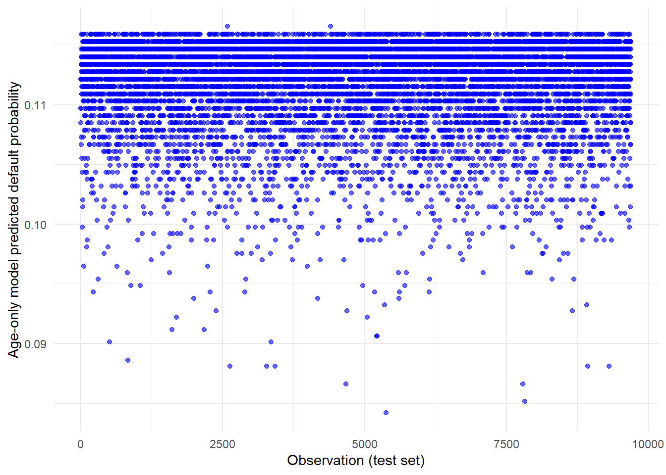
The points form a narrow horizontal band. This means that the age-only model assigns almost the same predicted default probability to many applicants, even though those applicants differ in other credit characteristics. A credit score can still be useful if its range is narrow but ranks borrowers well. Here, however, the narrow range reinforces the earlier warning from Figure 1.4. Age by itself is too weak to create meaningful default-risk separation.
The same predictions can also be viewed as a distribution.
Code
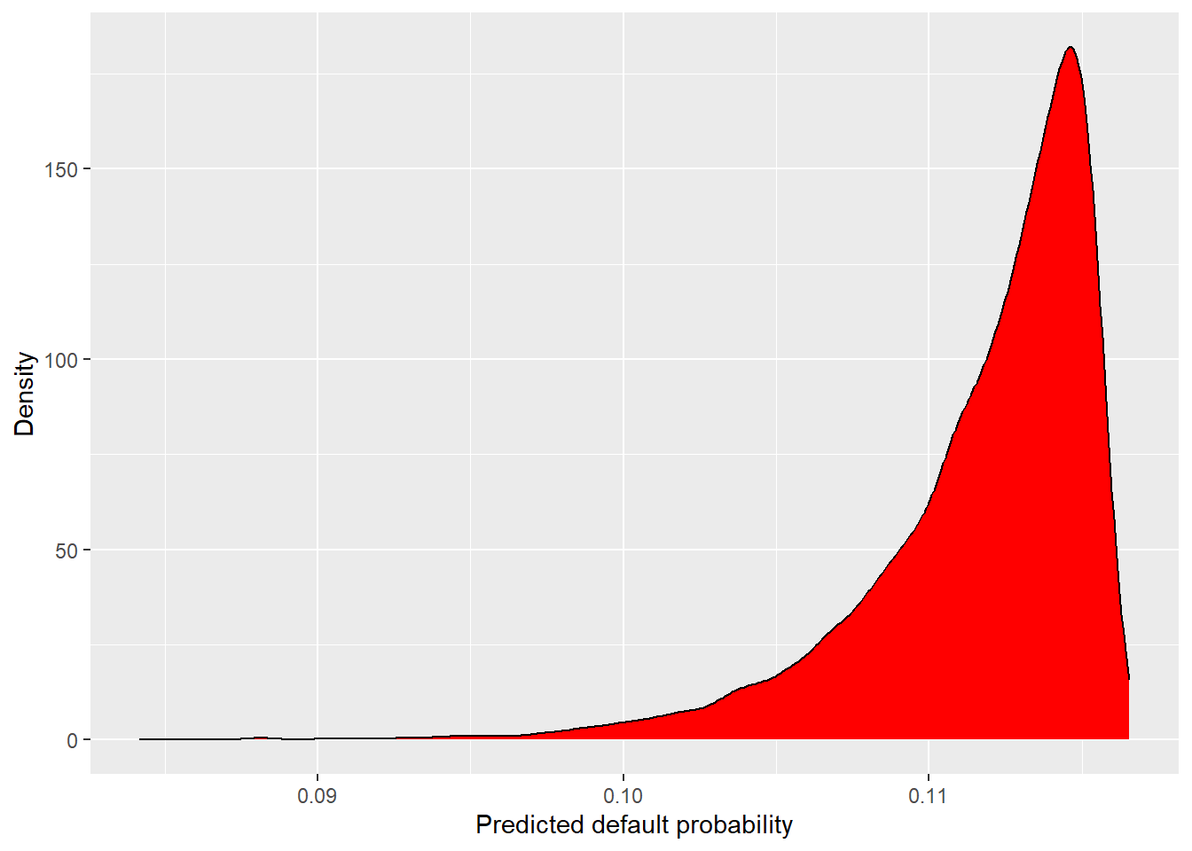
The logi_age predictions are concentrated in a very narrow probability range. A useful model can cover a limited interval, provided it still creates enough separation to rank applicants by risk. Here the age-only model assigns very similar predicted default probabilities to most applicants, so it has little ability to distinguish likely defaults from likely non-defaults.
The comparison now moves to logi_int and logi_multi. First, we collect the predictions in a single data frame.
The density plot shows how widely each model spreads predicted default probabilities.
Code
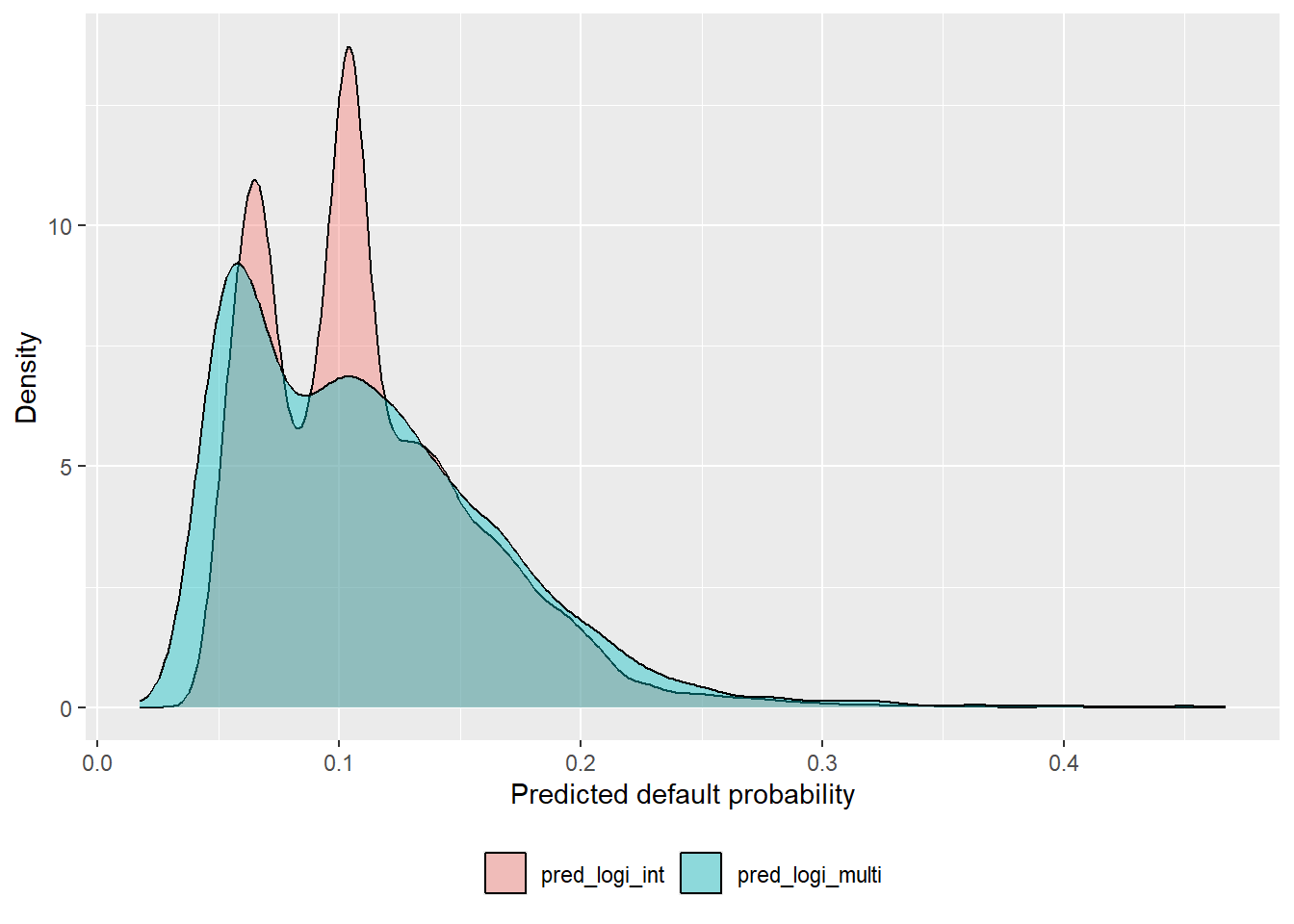
Adding the age model makes the contrast clearer.
Code
The previous section estimated logi_full, the most complete model in this chapter. Applying that model to the test set creates pred_logi_full, an object with one predicted default probability for each applicant in test.
Code
[1] 1.422469e-09 8.544424e-01Figure Figure 1.4 used age on the horizontal axis because the age-only model has only one predictor. The full model has many predictors, so age alone is no longer the right horizontal axis for the sigmoid. The natural horizontal axis is the full-model score, also called the logit score:
\[ \eta_i = \beta_0 + \beta_1 x_{1i} + \cdots + \beta_k x_{ki}. \]
This score combines age, interest rate, grade, loan amount, income, employment length, home ownership, sex, and region into one number. The model then converts that score into a predicted probability with the logistic function. In the test set, the full-model score ranges from -20.37 to 1.77, which maps to predicted default probabilities from 0.00% to 85.44%.
The direction of the curve is different from Figure 1.4 because the horizontal axis is different. In Figure 1.4, the horizontal axis is age and the estimated age coefficient is negative, -0.00623. As age increases, the age-only score decreases, so the predicted probability decreases. In Figure 1.9, the horizontal axis is the score \(\eta_i\) itself. The logistic transformation is increasing in \(\eta_i\), so moving to the right means a higher model score and therefore a higher predicted probability.
Code
ggplot(data = full_score_curve_data, aes(x = score, y = p)) +
  geom_line(color = "blue", linewidth = 2) +
  geom_segment(
    data = full_score_indicator_data,
    aes(x = score, xend = score, y = 0, yend = p),
    inherit.aes = FALSE,
    linetype = "dotted",
    linewidth = 0.9,
    color = "#C0392B"
  ) +
  geom_segment(
    data = full_score_indicator_data,
    aes(x = full_score_axis_min, xend = score, y = p, yend = p),
    inherit.aes = FALSE,
    linetype = "dotted",
    linewidth = 0.9,
    color = "#C0392B"
  ) +
  geom_segment(
    data = full_score_indicator_data,
    aes(x = score, xend = label_x, y = p, yend = label_y),
    inherit.aes = FALSE,
    linetype = "dotted",
    linewidth = 0.7,
    color = "#C0392B"
  ) +
  geom_point(
    data = full_score_indicator_data,
    aes(x = score, y = p),
    inherit.aes = FALSE,
    color = "#C0392B",
    size = 2.8
  ) +
  geom_label(
    data = full_score_indicator_data,
    aes(x = label_x, y = label_y, label = label),
    inherit.aes = FALSE,
    size = 3.2,
    fill = "white",
    color = "#7B241C",
    label.size = 0.2
  ) +
  scale_y_continuous(
    limits = c(0, 1),
    breaks = seq(0, 1, 0.25)
  ) +
  labs(x = "Full-model score (logit)", y = "Full-model predicted default probability") +
  theme_minimal()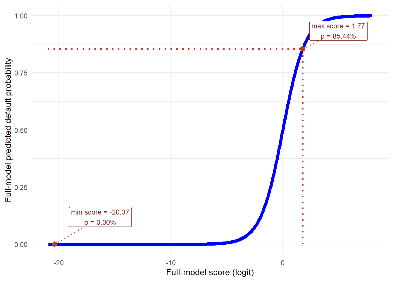
This figure should be read together with Figure 1.4. In the age-only model, the observed age range covers only a small and low-probability part of the sigmoid curve. In the full model, the combined score spans a much wider part of the same logistic transformation. That is why pred_logi_full can range from 0.00% to 85.44%. The wider range comes from the complete score, not from age by itself.
The right dotted point gives the highest predicted PD in the test set. Its score is \(\eta = 1.77\). Substituting that value into the logistic function gives:
\[ p = \frac{\exp(1.77)} {1+\exp(1.77)} = \frac{5.8701} {1+5.8701} = 0.8544 = 85.44%. \]
This calculation is the numerical bridge between the x-axis and the y-axis. The x-axis value is the full-model score. The y-axis value is the probability obtained after applying the logistic transformation.
The pred_logi_full prediction range is wider across the test set. Some applicants receive substantially higher predicted default probabilities than others, which can help the model separate likely defaults from likely non-defaults. A wider range is a useful sign, but classification and ranking metrics are needed before concluding that the model is better. The table below compares the prediction ranges across all models.
Code
pred_range <- rbind("logi_age" = range(pred_logi_age),
                     "logi_int" = range(pred_logi_int),
                     "logi_multi" = range(pred_logi_multi),
                     "logi_full" = range(pred_logi_full))
aic <- rbind(logi_age$aic, logi_int$aic, logi_multi$aic, logi_full$aic)
pred_range <- cbind(pred_range, aic)
colnames(pred_range) <- c("min(predicted PD)", "max(predicted PD)", "AIC")
pred_range_table <- data.frame(
  Model = rownames(pred_range),
  `Minimum predicted PD` = fmt_pct(pred_range[, "min(predicted PD)"], 2),
  `Maximum predicted PD` = fmt_pct(pred_range[, "max(predicted PD)"], 2),
  AIC = fmt_num(pred_range[, "AIC"], 1),
  row.names = NULL
)

knitr::kable(
  pred_range_table,
  caption = "Prediction ranges and AIC across logistic model candidates.",
  row.names = FALSE
)| Model | Minimum.predicted.PD | Maximum.predicted.PD | AIC |
|---|---|---|---|
| logi_age | 8.42% | 11.65% | 13580.7 |
| logi_int | 5.02% | 39.83% | 13215.6 |
| logi_multi | 1.74% | 46.68% | 13050.3 |
| logi_full | 0.00% | 85.44% | 10763.7 |
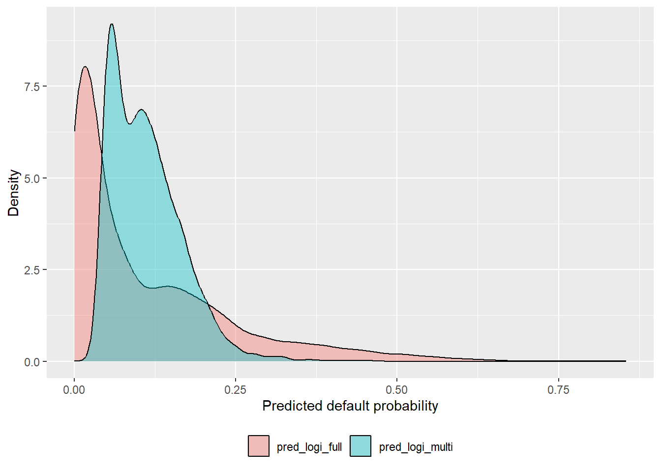
The next density plot compares the new pred_logi_full predictions with pred_logi_multi.
Code
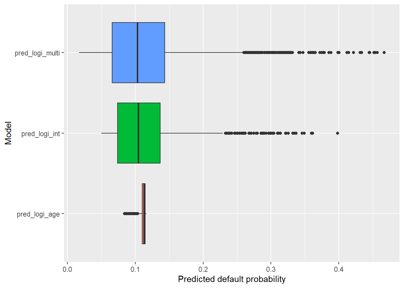
The boxplot adds all four models to the same comparison.
Code
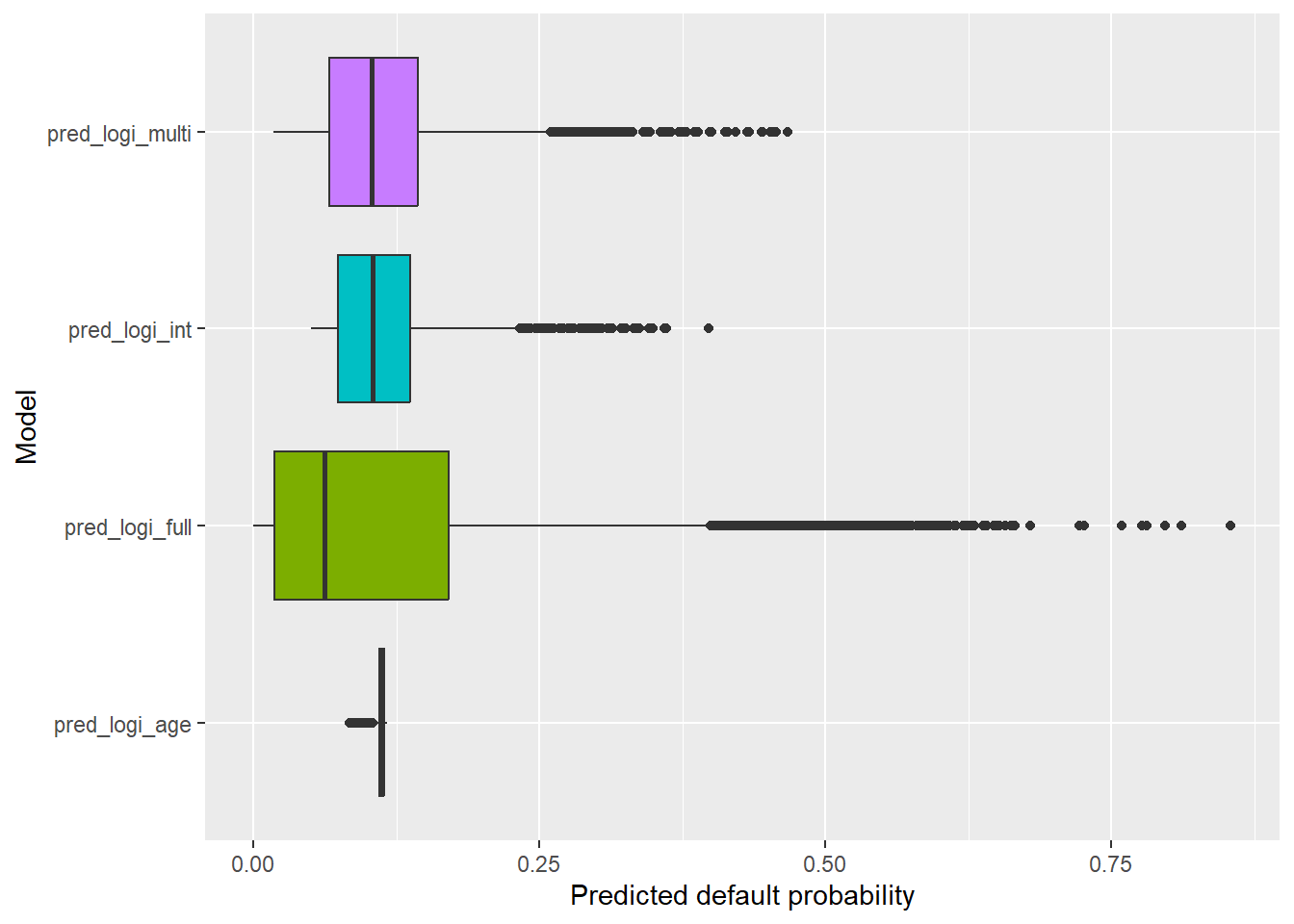
The logi_full predictions look more useful than the other models because they produce greater separation across applicants. The next question is whether this separation leads to better credit decisions.
To turn predicted probabilities into a lending decision, the bank needs a cutoff. The logi_full model produces predicted probabilities of default from 0.000 to 0.854. Denote the predicted probability for applicant \(i\) by \(\hat{p}_i = \widehat{P}(Y_i = 1 \mid x_i)\), where \(Y_i\) is the observed value stored in loan_st and \(x_i\) represents the applicant’s predictors. A cutoff \(c\) converts those probabilities into an accept/reject rule:
\[ \hat{y}_i(c) = \begin{cases} 1, & \text{if } \hat{p}_i > c \quad \text{predicted default, reject},\\ 0, & \text{if } \hat{p}_i \leq c \quad \text{predicted no default, accept}. \end{cases} \]
In code, the vector \(\hat p_i\) is pred_logi_full, the cutoff \(c\) is 0.15, and the binary decision \(\hat y_i(c)\) is pred_cutoff_15. The line ifelse(pred_logi_full > 0.15, 1, 0) is the direct code translation of this equation.
For a first pass, set a cutoff of 0.15. This teaching rule makes the conversion from probabilities to binary decisions explicit. Later in the chapter, we compare cutoff rules using confusion matrices, acceptance rates, bad rates, and financial payoff.
This 0.15 rule classifies any predicted probability below or equal to 0.15 as 0 (predicted no default) and any predicted probability above 0.15 as 1 (predicted default). In lending terms, applicants above the cutoff are rejected and applicants below or equal to the cutoff are accepted.
The cutoff is both a policy choice and a statistical choice. A higher cutoff accepts more applicants because more predicted probabilities fall below or equal to the cutoff. This can increase loan volume, but it can also accept more risky borrowers.
It is useful to distinguish two related but different cutoff ideas. A fixed probability cutoff, such as 0.15, represents an absolute risk tolerance. The bank accepts applicants only if their estimated probability of default is at most 15%. An acceptance-rate rule works differently. If the bank wants to accept 80% of applications, the cutoff is not chosen first; it is implied by the 80th percentile of the predicted probabilities. The first rule starts from a risk limit, while the second starts from a portfolio or business target.
Under the 0.15 rule, any predicted probability below or equal to 0.15 is classified as 0 (predicted no default), while any predicted probability above 0.15 is classified as 1 (predicted default). The cutoff is visible in the next scatter plot.
Code
# Convert the predictions to a data frame
cutoff_15 <- 0.15
cutoff_15_below <- mean(pred_logi_full <= cutoff_15)
cutoff_15_above <- mean(pred_logi_full > cutoff_15)

pred_data <- data.frame(
  Observation = seq_along(pred_logi_full),  # Sequence for observation index
  Predicted_Probabilities = pred_logi_full
)

cutoff_15_scatter_labels <- data.frame(
  x = length(pred_logi_full) * 0.72,
  y = c(cutoff_15 * 0.48,
        cutoff_15 + 0.68 * (max(pred_logi_full) - cutoff_15)),
  label = c(
    paste0("Accepted\n", fmt_pct(cutoff_15_below, 1)),
    paste0("Rejected\n", fmt_pct(cutoff_15_above, 1))
  )
)

# Create the plot
ggplot(pred_data, aes(x = Observation, y = Predicted_Probabilities)) +
  geom_point(alpha = 0.6, color = "blue") +  # Points for predictions
  geom_hline(yintercept = cutoff_15, color = "red", size = 1) +  # Horizontal line
  geom_label(
    data = cutoff_15_scatter_labels,
    aes(x = x, y = y, label = label),
    inherit.aes = FALSE,
    fill = "white",
    alpha = 0.92,
    label.size = 0,
    size = 3.5,
    lineheight = 0.95
  ) +
  labs(x = "Observation (test set)",
       y = "Full-model predicted default probability") +
  theme_minimal()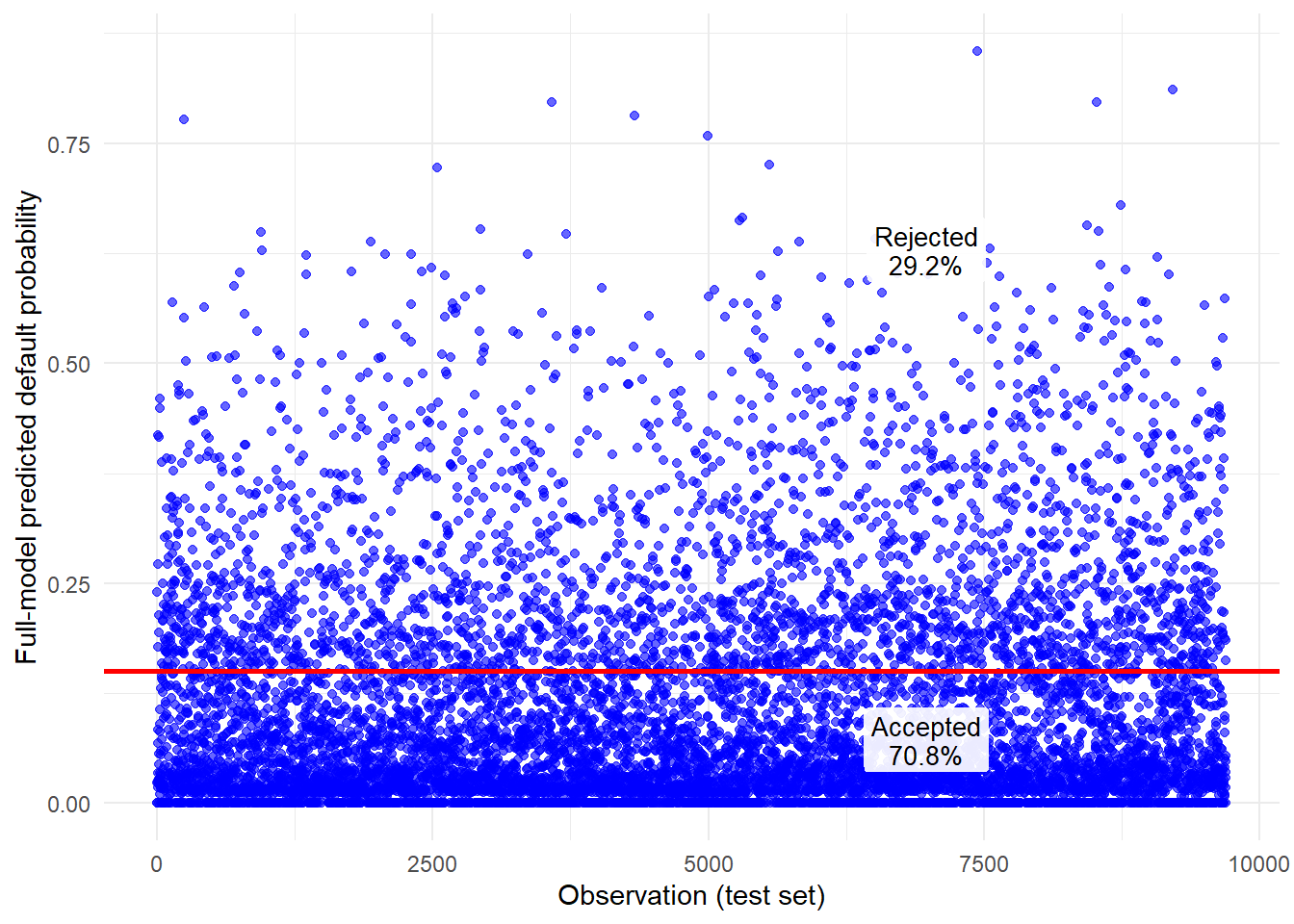
The distribution view gives the same rule from another angle.
Code
full_pred_density <- density(pred_logi_full)
cutoff_15_density_labels <- data.frame(
  x = c(cutoff_15 * 0.55,
        cutoff_15 + 0.48 * (max(pred_logi_full) - cutoff_15)),
  y = max(full_pred_density$y) * 0.82,
  label = c(
    paste0("Accepted\n", fmt_pct(cutoff_15_below, 1)),
    paste0("Rejected\n", fmt_pct(cutoff_15_above, 1))
  )
)

ggplot(pred_logi[pred_logi$model == "pred_logi_full",],
       aes(x = pred, fill = model)) +
  geom_density(alpha = 0.4) +
  geom_vline(xintercept = cutoff_15, linetype = "longdash", color = "red", linewidth = 0.8) +
  geom_label(
    data = cutoff_15_density_labels,
    aes(x = x, y = y, label = label),
    inherit.aes = FALSE,
    fill = "white",
    alpha = 0.92,
    label.size = 0,
    size = 3.4,
    lineheight = 0.95
  ) +
  labs(y = "Density", x = "Predicted default probability") +
  theme(legend.position = "none", legend.title = element_blank())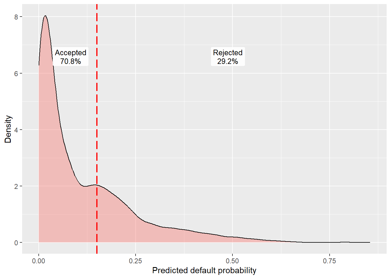
Predicted probabilities to the left of the dashed line are classified as no default. Predicted probabilities to the right are classified as default. The labels show the share of test-set applications on each side of the cutoff. The next code block creates that binary variable.
The next rows show the transformation from probability to binary prediction.
Code
# Make a binary predictions-vector using a cutoff of 15%
pred_cutoff_15 <- ifelse(pred_logi_full > 0.15, 1, 0)
cutoff_15_sample <- data.frame(
  `Predicted PD` = fmt_pct(head(pred_logi_full), 2),
  `Binary prediction` = head(pred_cutoff_15),
  `Credit decision` = ifelse(head(pred_cutoff_15) == 1, "Reject", "Accept")
)

knitr::kable(
  cutoff_15_sample,
  caption = "First six full-model predictions after applying the 15% cutoff.",
  row.names = FALSE
)| Predicted.PD | Binary.prediction | Credit.decision |
|---|---|---|
| 0.00% | 0 | Accept |
| 0.00% | 0 | Accept |
| 2.30% | 0 | Accept |
| 24.04% | 1 | Reject |
| 17.79% | 1 | Reject |
| 2.60% | 0 | Accept |
These are only the first 6 rows in the test set. The rule is doing exactly what the equation says. Every estimated default probability below or equal to 0.15 is coded as 0 (predicted no-default), and every estimated default probability above 0.15 is coded as 1 (predicted default). The table above shows the conversion from a probability, pred_logi_full, to a binary prediction, pred_cutoff_15.
The row numbers in the table above may be nonconsecutive because the test rows were selected randomly out of dat. They correspond to the original row positions in dat.
To see whether logi_full is making useful decisions, we compare predictions with realized outcomes. The first column is the logistic model prediction, the binary prediction applies the 0.15 cutoff, and the observed outcome tells us what happened historically. The final column translates the statistical classification into a lending consequence before we move to a full confusion matrix.
Code
# Take rows 101 to 110.
cutoff_15_observed_sample <- as.numeric(as.character(test$loan_st))[101:110]
cutoff_15_prediction_sample <- pred_cutoff_15[101:110]
cutoff_15_case_sample <- data.frame(
  `Application row` = rownames(test)[101:110],
  `Predicted PD` = fmt_pct(pred_logi_full[101:110], 2),
  `Binary prediction` = cutoff_15_prediction_sample,
  `Credit decision` = ifelse(cutoff_15_prediction_sample == 1, "Reject", "Accept"),
  `Observed outcome` = ifelse(cutoff_15_observed_sample == 1, "Default", "No default"),
  `Credit outcome` = ifelse(
    cutoff_15_prediction_sample == 0 & cutoff_15_observed_sample == 0,
    "Good loan accepted",
    ifelse(
      cutoff_15_prediction_sample == 0 & cutoff_15_observed_sample == 1,
      "Defaulting borrower accepted",
      ifelse(
        cutoff_15_prediction_sample == 1 & cutoff_15_observed_sample == 1,
        "Default avoided",
        "Good applicant rejected"
      )
    )
  ),
  check.names = FALSE
)

knitr::kable(
  cutoff_15_case_sample,
  caption = "Ten test-set cases comparing predicted PD, cutoff decision, observed outcome, and credit consequence.",
  row.names = FALSE
)| Application row | Predicted PD | Binary prediction | Credit decision | Observed outcome | Credit outcome |
|---|---|---|---|---|---|
| 308 | 15.37% | 1 | Reject | No default | Good applicant rejected |
| 309 | 4.14% | 0 | Accept | No default | Good loan accepted |
| 310 | 3.11% | 0 | Accept | No default | Good loan accepted |
| 312 | 0.00% | 0 | Accept | No default | Good loan accepted |
| 318 | 5.34% | 0 | Accept | No default | Good loan accepted |
| 319 | 8.40% | 0 | Accept | No default | Good loan accepted |
| 323 | 27.96% | 1 | Reject | Default | Default avoided |
| 328 | 0.00% | 0 | Accept | No default | Good loan accepted |
| 329 | 18.94% | 1 | Reject | No default | Good applicant rejected |
| 330 | 0.90% | 0 | Accept | No default | Good loan accepted |
1.5 Confusion matrices and bad rates
The previous section converted predicted probabilities into binary decisions through a cutoff. Those decisions can now be evaluated by comparing the predicted loan status with the actual loan status in the test set. The standard summary table is a confusion matrix.
A confusion matrix is useful only after a cutoff has been chosen. If the cutoff changes, the predicted 0/1 labels change, and the confusion matrix changes with them. For that reason, confusion matrices are helpful for evaluating a specific lending rule, but they are not an objective summary of the model by themselves. Later metrics such as ROC/AUC, calibration, and the Brier score evaluate prediction quality more systematically across cutoffs or directly on probabilities.
      Predicted
Actual    0    1
     0 6554 2081
     1  308  752
The logi_full model correctly predicts 6554 no-defaults and 752 defaults. It also misclassifies 2081 no-defaults as defaults and 308 defaults as no-defaults. In credit terms, the 2081 cases are good applicants that would be incorrectly rejected, while the 308 cases are bad applicants that would be incorrectly accepted. The sum of these four values equals 9695, the total number of observations in the test set.
Read the table by actual outcome. The row for actual no-defaults contains two groups. True negatives are correctly accepted as no-defaults, and false positives are incorrectly rejected as predicted defaults. In this cutoff rule, true negatives represent 67.6% of all test-set cases, while false positives represent 21.5%.
The row for actual defaults is the credit-risk row. True positives are defaults that the model correctly identifies and rejects; false negatives are defaults that the model misses and accepts. In this cutoff rule, true positives represent 7.8% of all test-set cases, while false negatives represent 3.2%. The false negatives are especially important for lending because they are accepted loans that later default.
The table also shows class imbalance. Non-defaults represent 89.1% of the test set, while defaults represent only 10.9%. This is why accuracy alone can be misleading.
Overall accuracy is defined as:
\[ \text{Accuracy} = \frac{\text{True negatives} + \text{True positives}} {\text{True negatives} + \text{False positives} + \text{False negatives} + \text{True positives}}. \]
In code, mean(pred_cutoff_15 == actual_default) computes the same quantity. It checks which binary predictions are equal to the observed outcomes and then averages the TRUE/FALSE values. This also shows why overall accuracy can be misleading in credit risk. Since most applicants in the test set do not default, a very naive rule that predicts “no default” for everyone can obtain a high accuracy simply by following the majority class. That rule would accept every loan that eventually defaults. A credit risk model should therefore be evaluated by the share of correct classifications and by the types of errors it makes.
Code
actual_default <- as.numeric(as.character(test$loan_st))
pred_all_no_default <- rep(0, length(actual_default))
pred_all_default <- rep(1, length(actual_default))

accuracy_summary <- data.frame(
  rule = c(
    "Full model with cutoff 0.15",
    "Always predict no default",
    "Always predict default"
  ),
  accuracy = c(
    mean(pred_cutoff_15 == actual_default),
    mean(pred_all_no_default == actual_default),
    mean(pred_all_default == actual_default)
  ),
  defaults_detected = c(
    sum(actual_default == 1 & pred_cutoff_15 == 1),
    sum(actual_default == 1 & pred_all_no_default == 1),
    sum(actual_default == 1 & pred_all_default == 1)
  ),
  accepted_defaults = c(
    sum(actual_default == 1 & pred_cutoff_15 == 0),
    sum(actual_default == 1 & pred_all_no_default == 0),
    sum(actual_default == 1 & pred_all_default == 0)
  )
)

accuracy_summary |>
  mutate(
    accuracy = fmt_pct(accuracy, 2),
    defaults_detected = fmt_int(defaults_detected),
    accepted_defaults = fmt_int(accepted_defaults)
  ) |>
  knitr::kable(
    caption = "Accuracy can reward poor credit-screening rules.",
    row.names = FALSE
)| rule | accuracy | defaults_detected | accepted_defaults |
|---|---|---|---|
| Full model with cutoff 0.15 | 75.36% | 752 | 308 |
| Always predict no default | 89.07% | 0 | 1,060 |
| Always predict default | 10.93% | 1,060 | 0 |
The always-no-default rule has higher accuracy, but it detects no defaults at all. This is unacceptable for credit screening because the bank would accept all defaulting applicants. The always-default rule detects every default, but it rejects every applicant and therefore creates no lending business. The full model with a cutoff of 0.15 sits between those extremes. It detects 752 defaults and reduces the number of defaulting loans accepted by the bank. In imbalanced classification problems, accuracy alone can reward the wrong behavior.
The 0.15 cutoff was a first teaching rule. A second approach starts from the bank’s desired acceptance rate. Suppose the bank wants to reject the 20% riskiest applicants and accept the remaining 80%. In that case, the cutoff should be the 80th percentile of pred_logi_full. Applicants above that cutoff are predicted defaults, and applicants below or equal to that cutoff are predicted no-defaults.
Code
[1] 0.1994621The conversion is direct. The desired acceptance rate is 80%, so we take the 80th percentile of the predicted default probabilities. In this test set, that percentile is 0.1994621, or 19.95%. The mapping is:
\[ \text{accept if } \hat p_i \leq 0.1994621, \qquad \text{reject if } \hat p_i > 0.1994621. \]
With this rule, 80.0% of applicants are accepted and 20.0% are rejected. The cutoff line is shown below.
Code
acceptance_density_labels <- data.frame(
  x = c(
    min(pred_logi_full) + 0.58 * (cutoff - min(pred_logi_full)),
    cutoff + 0.55 * (max(pred_logi_full) - cutoff)
  ),
  y = max(full_pred_density$y) * 0.82,
  label = c(
    paste0("Accepted\n", fmt_pct(acceptance_cutoff_below, 1)),
    paste0("Rejected\n", fmt_pct(acceptance_cutoff_above, 1))
  )
)

ggplot(pred_logi[pred_logi$model == "pred_logi_full",],
       aes(x = pred, fill = model)) +
  geom_density(alpha = 0.4) +
  geom_vline(xintercept = cutoff, linetype = "longdash", color = "red", linewidth = 0.8) +
  geom_label(
    data = acceptance_density_labels,
    aes(x = x, y = y, label = label),
    inherit.aes = FALSE,
    fill = "white",
    alpha = 0.92,
    label.size = 0,
    size = 3.4,
    lineheight = 0.95
  ) +
  labs(y = "Density", x = "Predicted default probability") +
  theme(legend.position = "none", legend.title = element_blank())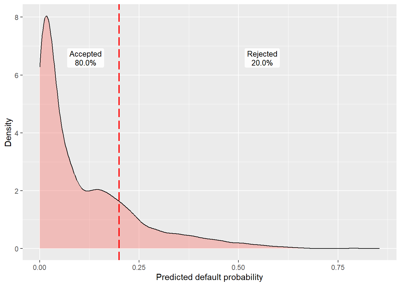
The cutoff is now 0.1994621. This splits the predicted default probabilities into two parts. Values above the cutoff are predicted defaults, and values below or equal to the cutoff are predicted no-defaults. The labels show the actual split in the test set. The next table reports cutoff values at several quantiles.
Code
cutoff_all <- quantile(pred_logi_full, seq(0.1, 1, 0.1))
cutoff_quantile_table <- data.frame(
  `Accepted share` = fmt_pct(seq(0.1, 1, 0.1), 0),
  `Cutoff` = fmt_pct(as.numeric(cutoff_all), 2)
)

knitr::kable(
  cutoff_quantile_table,
  caption = "Cutoffs implied by target acceptance rates.",
  row.names = FALSE
)| Accepted.share | Cutoff |
|---|---|
| 10% | 0.00% |
| 20% | 1.47% |
| 30% | 2.41% |
| 40% | 3.75% |
| 50% | 6.18% |
| 60% | 9.62% |
| 70% | 14.67% |
| 80% | 19.95% |
| 90% | 29.23% |
| 100% | 85.44% |
The same confusion-matrix logic now applies to the logi_full model with the new cutoff of 0.1994621.
Code
      Predicted
Actual    0    1
     0 7309 1326
     1  447  613
With a cutoff of 0.1994621, we accept 7309 + 447 = 7756 applications as those are the ones that the model predicts a no default. Previously, in the case of a cutoff of 0.15, we accepted 6554 + 308 = 6862.
The next table compares both confusion matrices.
Code
cat <- c("Correct no-default (true negatives).",
         "False default (false positives).",
         "False no-default (false negatives).",
         "Correct default (true positives).")
cut_15 <- fmt_pct(
  c(cm_cutoff_15["0", "0"], cm_cutoff_15["0", "1"],
    cm_cutoff_15["1", "0"], cm_cutoff_15["1", "1"]) /
    sum(cm_cutoff_15),
  1
)
cut_accept_80 <- fmt_pct(
  c(cm_full_20["0", "0"], cm_full_20["0", "1"],
    cm_full_20["1", "0"], cm_full_20["1", "1"]) /
    sum(cm_full_20),
  1
)
data.frame(
  classification = cat,
  cutoff_0_15 = cut_15,
  acceptance_80 = cut_accept_80
) |>
  knitr::kable(
    caption = "Classification outcomes under the 15% cutoff and the 80% acceptance rule.",
    row.names = FALSE
)| classification | cutoff_0_15 | acceptance_80 |
|---|---|---|
| Correct no-default (true negatives). | 67.6% | 75.4% |
| False default (false positives). | 21.5% | 13.7% |
| False no-default (false negatives). | 3.2% | 4.6% |
| Correct default (true positives). | 7.8% | 6.3% |
Type I and Type II errors are key concepts in hypothesis testing and statistical decision-making, particularly relevant in loan default prediction. A Type I error (false positive) occurs when good customers, who would not default, are incorrectly rejected. On the other hand, a Type II error (false negative) happens when bad customers, who will default, are mistakenly accepted.
The new cutoff of 0.1994621 improves the identification of no-defaults but worsens the identification of defaults. It creates fewer false positives and more false negatives, which is the central classification trade-off in this lending rule.
The next excerpt inspects individual cases under the 0.1994621 cutoff by comparing actual loan status with the binary prediction created from the estimated default probability.
Code
# Comparative table in detail.
real_pred_20 <- data.frame(
  observed_loan_status = test$loan_st,
  pred_full_20 = pred_full_20,
  "Did the model succeed?" = test$loan_st == pred_full_20,
  check.names = FALSE
)
# Show some values.
sample_real_pred_20 <- real_pred_20[131:140,]
sample_correct_rejections <- rownames(sample_real_pred_20)[
  sample_real_pred_20$pred_full_20 == 1 &
    sample_real_pred_20$observed_loan_status == 1
]
sample_lost_good_customers <- rownames(sample_real_pred_20)[
  sample_real_pred_20$pred_full_20 == 1 &
    sample_real_pred_20$observed_loan_status == 0
]
sample_model_failures <- sum(!sample_real_pred_20[["Did the model succeed?"]])
sample_real_pred_20 |>
  rename(
    `Observed outcome` = observed_loan_status,
    `Binary prediction` = pred_full_20
  ) |>
  knitr::kable(
    caption = "Sample of test-set outcomes under the 80% acceptance rule.",
    row.names = TRUE
)| Observed outcome | Binary prediction | Did the model succeed? | |
|---|---|---|---|
| 398 | 0 | 0 | TRUE |
| 399 | 1 | 1 | TRUE |
| 404 | 0 | 1 | FALSE |
| 414 | 0 | 0 | TRUE |
| 417 | 1 | 1 | TRUE |
| 419 | 0 | 0 | TRUE |
| 420 | 0 | 0 | TRUE |
| 425 | 1 | 1 | TRUE |
| 431 | 0 | 0 | TRUE |
| 435 | 0 | 0 | TRUE |
In this small excerpt, the model makes 1 mistake out of 10 applications. The acceptance rule is direct. If pred_full_20 = 0, the model predicts no default and the application is accepted. According to the excerpt, the model correctly rejects applications 399, 417, 425 because those were indeed defaults. It incorrectly rejects application 404, which did not default. The table makes the business meaning of the classification rule visible before we summarize all applications with aggregate metrics.
The aggregate count is simple.
Code
   total_applications accepted_applications rejected_applications
                 9695                  7756                  1939
By taking the top 20% of the pred_logi_full estimates as defaults and the bottom 80% as non-defaults, we construct a rule that accepts 7756 loan applications (80% of the total) and rejects 1939 applications (20% of the total). The cutoff criterion determines the number of accepted applications, while the logi_full model specifies which applications to accept or reject.
We evaluate the acceptance/rejection rule by comparing it against the actual outcomes recorded in loan_st. The next table combines the decision process with the ex-post evaluation.
Code
# First 12 accept/reject decisions.
head(data.frame(real_pred_20[,1:2],
                decision = ifelse(real_pred_20$pred_full_20 == 0,
                                  "accept", "reject"),
                evaluation =
                  ifelse(real_pred_20$pred_full_20 == 0 &
                           real_pred_20$observed_loan_status == 0,
                         "good decision",
                  ifelse(real_pred_20$pred_full_20 == 0 &
                           real_pred_20$observed_loan_status == 1,
                         "bad decision",
                  ifelse(real_pred_20$pred_full_20 == 1 &
                           real_pred_20$observed_loan_status == 1,
                         "correct rejection",
                         "lost good customer")))), 12) |>
  rename(
    `Observed outcome` = observed_loan_status,
    `Binary prediction` = pred_full_20,
    Decision = decision,
    Evaluation = evaluation
  ) |>
  knitr::kable(
    caption = "First 12 accept/reject decisions with ex-post evaluation.",
    row.names = FALSE
)| Observed outcome | Binary prediction | Decision | Evaluation |
|---|---|---|---|
| 0 | 0 | accept | good decision |
| 0 | 0 | accept | good decision |
| 1 | 0 | accept | bad decision |
| 0 | 1 | reject | lost good customer |
| 0 | 0 | accept | good decision |
| 0 | 0 | accept | good decision |
| 0 | 0 | accept | good decision |
| 0 | 0 | accept | good decision |
| 0 | 1 | reject | lost good customer |
| 0 | 0 | accept | good decision |
| 0 | 0 | accept | good decision |
| 1 | 0 | accept | bad decision |
The table shows the outcomes of the first 12 loan applications. A “good decision” means the bank accepts a loan that does not default. A “bad decision” means the bank accepts a loan that defaults. A correct rejection avoids a defaulting borrower. A lost good customer is an applicant who would not have defaulted but is rejected by the model rule.
Because this is a historical test set, we can observe the true loan_st for every applicant in the sample. That lets us evaluate accepted and rejected cases after the fact. In a live lending process, a rejected applicant usually does not become a loan in the bank’s own portfolio, so the bank does not observe that applicant’s repayment behavior as one of its borrowers. For operating a credit policy, the most immediate question is focused on the loans the bank actually accepts. Among accepted loans, how many default? This is the bad rate.
The real_pred_20 object contains both the binary model predictions and the actual loan status. In the code below, we first filter for accepted loans, which are cases where the prediction equals 0. If this condition is met, we keep the value from the first column, which is the observed loan status.
As a result, accepted_loans becomes a vector of zeros and ones. A value of 0 indicates a loan that did not default, while a value of 1 indicates a loan that defaulted. The length of the accepted_loans vector corresponds to the number of loans allocated based on the cutoff value of 0.1994621 and the predictions from the logi_full model.
For a cutoff \(c\), the rule above already tells us which loans are accepted. A loan is accepted when \(\hat y_i(c)=0\). The bad rate is simply:
\[ \text{bad rate}(c) = \frac{\text{accepted loans that default}} {\text{accepted loans}}, \]
where default means \(y_i=1\). In the code below, pred_full_20 == 0 finds the accepted applications, accepted_loans <- real_pred_20$observed_loan_status[pred_full_20 == 0] keeps their observed outcomes, sum(accepted_loans == 1) counts the accepted loans that default, and length(accepted_loans) counts all accepted loans.
Code
# We accept loans that the model predicts a no-default (0).
# In "accepted_loans" we know whether the accepted loans are in fact
# default or no-default.
accepted_index <- which(pred_full_20 == 0)
accepted_loans <- as.numeric(as.character(real_pred_20$observed_loan_status[accepted_index]))
# The code above says: if we accept the application, tell me what happened.
length(accepted_loans)
[1] 7756Code
accepted_sample_index <- head(accepted_index, 10)
accepted_sample <- data.frame(
  `Application row` = rownames(real_pred_20)[accepted_sample_index],
  `Predicted PD` = fmt_pct(pred_logi_full[accepted_sample_index], 2),
  `Binary prediction` = pred_full_20[accepted_sample_index],
  Decision = "accept",
  `Observed outcome` = ifelse(
    accepted_loans[seq_along(accepted_sample_index)] == 1,
    "default",
    "no default"
  ),
  check.names = FALSE
)

knitr::kable(
  accepted_sample,
  caption = "First 10 accepted applications and their observed outcomes.",
  row.names = FALSE
)| Application row | Predicted PD | Binary prediction | Decision | Observed outcome |
|---|---|---|---|---|
| 1 | 0.00% | 0 | accept | no default |
| 2 | 0.00% | 0 | accept | no default |
| 18 | 2.30% | 0 | accept | default |
| 27 | 17.79% | 0 | accept | no default |
| 28 | 2.60% | 0 | accept | no default |
| 30 | 3.39% | 0 | accept | no default |
| 32 | 8.32% | 0 | accept | no default |
| 35 | 1.77% | 0 | accept | no default |
| 36 | 2.36% | 0 | accept | no default |
| 37 | 6.80% | 0 | accept | default |
The small excerpt above shows individual accepted loans and their outcomes. The full bad-rate calculation uses all 7,756 accepted loans:
Code
# bad_rate is the proportion of accepted loans that are in fact default.
bad_rate_80 <- sum(accepted_loans == 1) / length(accepted_loans)
knitr::kable(
  data.frame(
    Quantity = c("Accepted defaults", "Accepted applications", "Bad rate"),
    Value = c(
      fmt_int(sum(accepted_loans == 1)),
      fmt_int(length(accepted_loans)),
      fmt_pct(bad_rate_80, 2)
    )
  ),
  caption = "Bad rate among accepted loans at the 80% acceptance rule.",
  row.names = FALSE
)| Quantity | Value |
|---|---|
| Accepted defaults | 447 |
| Accepted applications | 7,756 |
| Bad rate | 5.76% |
Following the model-based rule, we accepted 7756 loan applications, which represent 80% of all applications. Among those accepted applications, 5.76% were in fact defaults. In counts, we accepted 447 loans that defaulted, so 447 / 7756 = 0.0576328.
The bank can lower the bad rate by becoming more selective. With the same model, that means lowering the acceptance rate and approving fewer applications. This reduces credit risk, but it can also reduce business volume because the bank rejects more potential customers.
Reducing the acceptance rate from 80% to 65% shows how the bad rate changes when the bank becomes more selective.
Code
# New cutoff value.
cutoff <- quantile(pred_logi_full, 0.65)
# Split the pred_logi_full into a binary variable.
pred_full_35 <- ifelse(pred_logi_full > cutoff, 1, 0)
# A data frame with real and predicted loan status.
real_pred_35 <- data.frame(
  observed_loan_status = test$loan_st,
  pred_full_35 = pred_full_35
)
# Loans that we accept given these new rules.
accepted_loans <- real_pred_35[pred_full_35 == 0, 1]
# Bad rate (accepted loan applications that are defaults).
bad_rate_65 <- sum(accepted_loans == 1)/length(accepted_loans)
knitr::kable(
  data.frame(
    Quantity = c("Accepted defaults", "Accepted applications", "Bad rate"),
    Value = c(
      fmt_int(sum(accepted_loans == 1)),
      fmt_int(length(accepted_loans)),
      fmt_pct(bad_rate_65, 2)
    )
  ),
  caption = "Bad rate among accepted loans at the 65% acceptance rule.",
  row.names = FALSE
)| Quantity | Value |
|---|---|
| Accepted defaults | 234 |
| Accepted applications | 6,302 |
| Bad rate | 3.71% |
The bad rate falls from 5.76% to 3.71% when the acceptance rate is reduced from 80% to 65%. This illustrates the trade-off. A lower acceptance rate usually means fewer accepted defaults and fewer accepted customers. In the extreme, accepting 0 applications would produce a bad rate of zero and no loan business at all. The next section evaluates this trade-off across many acceptance rates after the two benchmark cases, 80% and 65%.
1.6 Acceptance strategy and model comparison
A bank needs to understand how the bad rate changes when it accepts more or fewer applications. The previous section compared two acceptance rates, 80% and 65%. We now evaluate the same idea over a wider grid of acceptance rates.
Once this trade-off is clear, the bank could move beyond a single accept/reject cutoff. For example, it could create risk bands. Low-risk applicants are accepted at standard terms, medium-risk applicants are accepted with a higher interest rate or additional conditions, and high-risk applicants are rejected. The simple accept/reject rule below is the first step because it makes the mechanics visible.
Code
bank <- function(prob_of_default, actual_default) {
  actual_default <- as.numeric(as.character(actual_default))

  # Pre-define the acceptance rates
  accept_rate <- seq(1, 0, by = -0.05)

  # Calculate cutoffs for each acceptance rate
  cutoff <- quantile(prob_of_default, accept_rate)

  # Calculate bad rates for each cutoff
  bad_rate <- sapply(cutoff, function(thresh) {
    accepted <- prob_of_default <= thresh
    mean(actual_default[accepted] == 1)
  })

  # Create the result table
  table <- cbind(
    accept_rate,
    cutoff = round(cutoff, 4),
    bad_rate = round(bad_rate, 4)
  )

  return(list(table = table, bad_rate = bad_rate, accept_rate = accept_rate, cutoff = cutoff))
}
The function receives two inputs. The first input is the vector of predicted probabilities, such as pred_logi_full. The second input is the observed loan outcome, test$loan_st, which is needed to calculate how many accepted loans actually default. Evaluating this function for logi_full and logi_age lets us compare a stronger model with a weaker benchmark. A stronger model should produce lower bad rates for the same acceptance rate.
The next code applies the function to pred_logi_full and pred_logi_age.
Code
# Apply the bank function.
bank_logi_full <- bank(pred_logi_full, test$loan_st)
bank_logi_age <- bank(pred_logi_age, test$loan_st)

data.frame(
  `Acceptance rate` = fmt_pct(bank_logi_age$accept_rate, 0),
  `Age-only bad rate` = fmt_pct(bank_logi_age$bad_rate, 2),
  `Full-model bad rate` = fmt_pct(bank_logi_full$bad_rate, 2),
  check.names = FALSE
) |>
  knitr::kable(
    caption = "Bad rate by acceptance rate for the age-only and full logistic models.",
    row.names = FALSE
)| Acceptance rate | Age-only bad rate | Full-model bad rate |
|---|---|---|
| 100% | 10.93% | 10.93% |
| 95% | 10.85% | 9.07% |
| 90% | 10.85% | 7.68% |
| 85% | 10.85% | 6.66% |
| 80% | 10.55% | 5.76% |
| 75% | 10.55% | 5.06% |
| 70% | 10.40% | 4.36% |
| 65% | 10.40% | 3.71% |
| 60% | 10.09% | 2.94% |
| 55% | 10.09% | 2.34% |
| 50% | 9.93% | 2.10% |
| 45% | 10.21% | 1.86% |
| 40% | 10.21% | 1.55% |
| 35% | 9.91% | 1.18% |
| 30% | 9.97% | 0.93% |
| 25% | 10.34% | 0.54% |
| 20% | 9.72% | 0.36% |
| 15% | 9.36% | 0.14% |
| 10% | 10.13% | 0.00% |
| 5% | 10.52% | 0.00% |
| 0% | 0.00% | 0.00% |
The table suggests that the full model is more useful for decision-making because it achieves a lower bad rate at any given acceptance rate. The next plot highlights the key differences between logi_age and logi_full.
Code
# Combine the two datasets for easier comparison
bank_logi_full$model <- "logi_full"
bank_logi_age$model <- "logi_age"
combined_data <- bind_rows(bank_logi_full, bank_logi_age)

# Add vertical and horizontal lines for visualization
highlight_lines <- tibble(
  model = c("logi_full", "logi_full", "logi_age", "logi_age"),
  accept_rate = c(bank_logi_full[["accept_rate"]][8],
                  bank_logi_full[["accept_rate"]][5],
                  bank_logi_age[["accept_rate"]][8],
                  bank_logi_age[["accept_rate"]][5]),
  bad_rate = c(bank_logi_full[["bad_rate"]][8],
               bank_logi_full[["bad_rate"]][5],
               bank_logi_age[["bad_rate"]][8],
               bank_logi_age[["bad_rate"]][5]),
  color = c("black", "red", "black", "red")
)

# Add a color column to distinguish facets
combined_data <- combined_data %>%
  mutate(facet_color = ifelse(model == "logi_full", "blue", "orange"))

ggplot(combined_data, aes(x = accept_rate, y = bad_rate, color = facet_color)) +
  geom_line(linewidth = 1.7) +  # Use facet-specific colors for the lines
  geom_vline(data = highlight_lines, aes(xintercept = accept_rate, color = color),
             linetype = "dashed", linewidth = 0.65) +
  geom_hline(data = highlight_lines, aes(yintercept = bad_rate, color = color),
             linetype = "dashed", linewidth = 0.65) +
  facet_wrap(~model, nrow = 1, scales = "free_y") +
  labs(x = "Acceptance rate", y = "Bad rate") +
  theme_minimal(base_size = 14) +
  theme(legend.position = "none") +
  scale_color_identity() +  # Use the colors directly without adding them to the legend
  scale_x_continuous(breaks = c(0, 0.65, 0.8, 1)) +
  scale_y_continuous(
    labels = function(x) fmt_pct(x, 0),
    breaks = scales::breaks_pretty(n = 5)
  )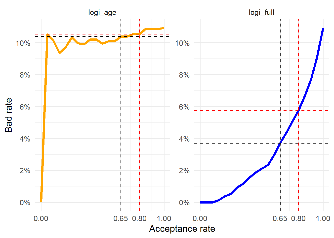
The plot reinforces the same conclusion. At the same acceptance rate, logi_full produces a lower bad rate than logi_age. The two panels use separate vertical scales so the age-only curve remains readable even though its bad-rate values are very close to each other. The value of a stronger model lies in its capacity to support better business decisions, in this case, more accurate credit evaluations.
The bad rate is useful, but it only describes part of the business decision. A very restrictive strategy can produce a low bad rate by rejecting many applicants, including many applicants who would have repaid their loans. To connect the model with a simple decision criterion, we define a hypothetical net payoff. It should be read as a transparent scoring rule, with accepting a good loan treated as a benefit and accepting a bad loan treated as a cost.
Suppose that accepting a loan that does not default gives the bank a payoff of $1, while accepting a loan that defaults costs $5. Rejected loans receive a payoff of $0 because the bank does not issue the loan. Under these assumptions:
\[ \text{net payoff} = (\text{accepted good loans}) \times \text{\$1} - (\text{accepted default loans}) \times \text{\$5}. \]
In the code below, accepted_good is the first term, accepted_defaults is the second term, good_loan_payoff = 1 represents $1, and bad_loan_cost = 5 represents $5. The expression accepted_good * good_loan_payoff - accepted_defaults * bad_loan_cost is therefore the code version of the equation. This lets us compare acceptance rates using the same model and the same test set.
Code
actual_default_strategy <- as.numeric(as.character(test$loan_st))

net_payoff_strategy <- function(prob_of_default, accept_rate,
                                good_loan_payoff = 1,
                                bad_loan_cost = 5) {
  cutoff <- unname(quantile(prob_of_default, accept_rate))
  accept <- prob_of_default <= cutoff
  accepted_good <- sum(actual_default_strategy[accept] == 0)
  accepted_defaults <- sum(actual_default_strategy[accept] == 1)
  accepted <- sum(accept)
  net_payoff <- accepted_good * good_loan_payoff -
    accepted_defaults * bad_loan_cost

  data.frame(
    accept_rate = accept_rate,
    cutoff = cutoff,
    accepted = accepted,
    accepted_good = accepted_good,
    accepted_defaults = accepted_defaults,
    bad_rate = accepted_defaults / accepted,
    net_payoff = net_payoff
  )
}

acceptance_grid <- c(0.50, 0.60, 0.65, 0.70, 0.75, 0.80, 0.85, 0.90)
net_payoff_results <- do.call(
  rbind,
  lapply(acceptance_grid, net_payoff_strategy,
         prob_of_default = pred_logi_full)
)

best_net_payoff_row <- net_payoff_results[
  which.max(net_payoff_results$net_payoff),
]

fmt_dollar <- function(x) {
  paste0(ifelse(x < 0, "-$", "$"), fmt_int(abs(x)))
}

net_payoff_results |>
  mutate(
    cutoff = round(cutoff, 4),
    bad_rate = fmt_pct(bad_rate, 2),
    net_payoff = fmt_dollar(net_payoff)
  ) |>
  knitr::kable(
    caption = "Net payoff across acceptance rates for the full logistic model.",
    row.names = FALSE
)| accept_rate | cutoff | accepted | accepted_good | accepted_defaults | bad_rate | net_payoff |
|---|---|---|---|---|---|---|
| 0.50 | 0.0618 | 4848 | 4746 | 102 | 2.10% | $4,236 |
| 0.60 | 0.0962 | 5817 | 5646 | 171 | 2.94% | $4,791 |
| 0.65 | 0.1223 | 6302 | 6068 | 234 | 3.71% | $4,898 |
| 0.70 | 0.1467 | 6786 | 6490 | 296 | 4.36% | $5,010 |
| 0.75 | 0.1711 | 7271 | 6903 | 368 | 5.06% | $5,063 |
| 0.80 | 0.1995 | 7756 | 7309 | 447 | 5.76% | $5,074 |
| 0.85 | 0.2342 | 8240 | 7691 | 549 | 6.66% | $4,946 |
| 0.90 | 0.2923 | 8725 | 8055 | 670 | 7.68% | $4,705 |
The table contains the complete payoff calculation, but the best row is worth checking explicitly. At the selected acceptance rate, the rule accepts 7309 good loans and 447 defaulting loans. Under the assumed payoffs, the calculation is:
\[ 7309(\text{\$1}) - 447(\text{\$5}) = \text{\$5,074}. \]
Code
best_net_payoff_check <- data.frame(
  Quantity = c(
    "Acceptance rate",
    "Accepted good loans",
    "Payoff from good loans ($1 each)",
    "Accepted default loans",
    "Cost from default loans ($5 each)",
    "Net payoff"
  ),
  Value = c(
    fmt_pct(best_net_payoff_row$accept_rate, 0),
    fmt_int(best_net_payoff_row$accepted_good),
    fmt_dollar(best_net_payoff_row$accepted_good * 1),
    fmt_int(best_net_payoff_row$accepted_defaults),
    fmt_dollar(-best_net_payoff_row$accepted_defaults * 5),
    fmt_dollar(best_net_payoff_row$net_payoff)
  )
)

knitr::kable(
  best_net_payoff_check,
  caption = "Numerical check of the best net-payoff row.",
  row.names = FALSE
)| Quantity | Value |
|---|---|
| Acceptance rate | 80% |
| Accepted good loans | 7,309 |
| Payoff from good loans ($1 each) | $7,309 |
| Accepted default loans | 447 |
| Cost from default loans ($5 each) | -$2,235 |
| Net payoff | $5,074 |
In this example, the highest net payoff occurs at an acceptance rate of 80%. The result is specific to this payoff assumption. The additional good loans accepted when moving from 65% to 80% more than compensate for the additional defaults. After 80%, accepting more applications still brings in more good loans, but the extra defaults become too costly under this rule.
The preferred acceptance rate depends on how costly defaults are relative to good accepted loans. The calculation can therefore be repeated under different assumptions for the cost of accepting a default.
Code
best_net_payoff <- function(bad_loan_cost) {
  payoff_grid <- do.call(
    rbind,
    lapply(seq(0.50, 0.95, 0.05), net_payoff_strategy,
           prob_of_default = pred_logi_full,
           bad_loan_cost = bad_loan_cost)
  )

  payoff_grid[which.max(payoff_grid$net_payoff), ]
}

net_payoff_sensitivity <- do.call(
  rbind,
  lapply(c(2, 5, 10, 15), best_net_payoff)
)

data.frame(
  bad_loan_cost = fmt_dollar(c(2, 5, 10, 15)),
  best_accept_rate = net_payoff_sensitivity$accept_rate,
  accepted_defaults = net_payoff_sensitivity$accepted_defaults,
  bad_rate = net_payoff_sensitivity$bad_rate,
  net_payoff = fmt_dollar(net_payoff_sensitivity$net_payoff)
) |>
  mutate(
    best_accept_rate = fmt_pct(best_accept_rate, 0),
    accepted_defaults = fmt_int(accepted_defaults),
    bad_rate = fmt_pct(bad_rate, 2)
  ) |>
  knitr::kable(
    caption = "Net-payoff sensitivity to the cost of accepting a default.",
    row.names = FALSE
)| bad_loan_cost | best_accept_rate | accepted_defaults | bad_rate | net_payoff |
|---|---|---|---|---|
| $2 | 90% | 670 | 7.68% | $6,715 |
| $5 | 80% | 447 | 5.76% | $5,074 |
| $10 | 55% | 125 | 2.34% | $3,957 |
| $15 | 55% | 125 | 2.34% | $3,332 |
The sensitivity table shows the economic intuition. If accepting a default is relatively less costly, the strategy can tolerate a higher acceptance rate. If accepting a default is much more costly, the strategy becomes more conservative. The assumed payoffs are a transparent cost-benefit exercise for cutoff selection, not real bank profits.
This simple net payoff rule is closely related to the credit-risk idea of expected loss. A standard expected-loss expression is:
\[ \text{Expected loss} = PD \times LGD \times EAD, \]
where \(PD\) is the probability of default, \(LGD\) is loss given default, and \(EAD\) is exposure at default. In this chapter, the predicted probability \(\hat p_i\) plays the role of the model-based \(PD\), while $1 and $5 are simplified teaching assumptions about benefits and costs. A full profitability model would also include loan amount, interest income, funding costs, recovery rates, and exposure. The simplified net payoff is a first cost-benefit version of the same decision logic before adding those additional banking details.
1.7 ROC, AUC, and calibration
Before introducing ROC curves, we need to fix the classification language. In this chapter, the positive class is default. A predicted positive is therefore a predicted default, which means the lending rule rejects the applicant. A predicted negative is a predicted no-default, which means the lending rule accepts the applicant.
Code
classification_equivalence_table <- data.frame(
  `Actual outcome` = c(
    "No default",
    "No default",
    "Default",
    "Default"
  ),
  `Model prediction` = c(
    "No default",
    "Default",
    "No default",
    "Default"
  ),
  `Statistical name` = c(
    "True negative (TN)",
    "False positive (FP)",
    "False negative (FN)",
    "True positive (TP)"
  ),
  `Credit reading` = c(
    "The model expected repayment, and the borrower repaid.",
    "The model expected default, but the borrower would have repaid.",
    "The model expected repayment, but the borrower defaulted.",
    "The model expected default, and the borrower defaulted."
  ),
  `Lending consequence` = c(
    "Good loan accepted",
    "Good applicant rejected",
    "Defaulting borrower accepted",
    "Default avoided"
  ),
  check.names = FALSE
)

knitr::kable(
  classification_equivalence_table,
  caption = "Confusion-matrix language translated into credit decisions.",
  row.names = FALSE
)| Actual outcome | Model prediction | Statistical name | Credit reading | Lending consequence |
|---|---|---|---|---|
| No default | No default | True negative (TN) | The model expected repayment, and the borrower repaid. | Good loan accepted |
| No default | Default | False positive (FP) | The model expected default, but the borrower would have repaid. | Good applicant rejected |
| Default | No default | False negative (FN) | The model expected repayment, but the borrower defaulted. | Defaulting borrower accepted |
| Default | Default | True positive (TP) | The model expected default, and the borrower defaulted. | Default avoided |
The table is useful because the words positive and negative can be misleading in credit risk. Positive does not mean good. It means that the event of interest occurred, and here the event of interest is default. A false negative is therefore costly for the lender because the model accepts a borrower who defaults. A false positive is also costly, but in a different way, because the bank rejects a borrower who would have repaid.
The same language gives the four rates used in ROC analysis.
Code
classification_metric_table <- data.frame(
  Metric = c(
    "Sensitivity",
    "Specificity",
    "False positive rate",
    "False negative rate"
  ),
  Formula = c(
    "$TP/(TP+FN)$",
    "$TN/(TN+FP)$",
    "$FP/(TN+FP)=1-\\text{specificity}$",
    "$FN/(TP+FN)=1-\\text{sensitivity}$"
  ),
  `Credit meaning` = c(
    "Among actual defaults, the share correctly detected as predicted defaults.",
    "Among actual non-defaults, the share correctly kept as predicted no-defaults.",
    "Among good borrowers, the share wrongly rejected.",
    "Among defaulting borrowers, the share wrongly accepted."
  ),
  check.names = FALSE
)

knitr::kable(
  classification_metric_table,
  caption = "Sensitivity, specificity, and error rates in credit language.",
  row.names = FALSE,
  escape = FALSE
)| Metric | Formula | Credit meaning |
|---|---|---|
| Sensitivity | \(TP/(TP+FN)\) | Among actual defaults, the share correctly detected as predicted defaults. |
| Specificity | \(TN/(TN+FP)\) | Among actual non-defaults, the share correctly kept as predicted no-defaults. |
| False positive rate | \(FP/(TN+FP)=1-\text{specificity}\) | Among good borrowers, the share wrongly rejected. |
| False negative rate | \(FN/(TP+FN)=1-\text{sensitivity}\) | Among defaulting borrowers, the share wrongly accepted. |
The acceptance-rate analysis compares business rules at selected cutoffs. The next metrics summarize ranking, calibration, and sensitivity/specificity across cutoffs. The ROC (Receiver Operating Characteristic) curve evaluates how well the model ranks defaults above non-defaults as the cutoff changes.
Throughout this book, we draw ROC curves with sensitivity on the vertical axis and the false positive rate on the horizontal axis. The false positive rate is \(1 - \text{specificity}\). In credit terms, it is the share of non-default loans that the model incorrectly classifies as predicted defaults at a given cutoff. This convention matches the ROC figures used in the next chapter.
The area under the ROC curve (AUC) quantifies the model’s ability to discriminate between the two classes. A higher AUC indicates better ranking performance. For example, a model with an AUC close to 1 tends to assign higher default probabilities to defaulting borrowers than to non-defaulting borrowers, while an AUC of 0.5 indicates no better ranking performance than random guessing. By analyzing the trade-off between sensitivity (correctly identifying defaults) and specificity (correctly identifying non-defaults), the ROC curve helps determine an operational threshold for classification, balancing the cost of misclassifying borrowers.
Code
# Calculate ROC curves
ROC_logi_full <- roc(test$loan_st, pred_logi_full, quiet = TRUE)
ROC_logi_age <- roc(test$loan_st, pred_logi_age, quiet = TRUE)
auc_logi_full <- as.numeric(auc(ROC_logi_full))
auc_logi_age <- as.numeric(auc(ROC_logi_age))

roc_to_df_logistic <- function(roc_object, model_name) {
  data.frame(
    false_positive_rate = 1 - roc_object$specificities,
    true_positive_rate = roc_object$sensitivities,
    model = model_name,
    auc = as.numeric(auc(roc_object))
  )
}

roc_logistic_comparison <- bind_rows(
  roc_to_df_logistic(ROC_logi_full, "logi_full"),
  roc_to_df_logistic(ROC_logi_age, "logi_age")
) |>
  mutate(
    model_label = paste0(model, " (AUC = ", fmt_num(auc, 4), ")"),
    model_label = factor(model_label, levels = unique(model_label))
  ) |>
  arrange(model_label, false_positive_rate)

ggplot(
  roc_logistic_comparison,
  aes(x = false_positive_rate, y = true_positive_rate, color = model_label)
) +
  geom_abline(
    intercept = 0,
    slope = 1,
    linetype = "dashed",
    color = "gray60",
    linewidth = 0.7
  ) +
  geom_line(linewidth = 1.2) +
  scale_color_manual(
    values = c("blue", "orange"),
    name = NULL
  ) +
  scale_x_continuous(
    labels = scales::percent_format(accuracy = 1),
    limits = c(0, 1),
    expand = c(0.01, 0.01)
  ) +
  scale_y_continuous(
    labels = scales::percent_format(accuracy = 1),
    limits = c(0, 1),
    expand = c(0.01, 0.01)
  ) +
  labs(
    x = "False positive rate (1 - specificity)",
    y = "True positive rate (sensitivity)"
  ) +
  coord_equal() +
  theme_minimal() +
  theme(
    legend.position = "bottom",
    panel.grid.minor = element_blank()
  )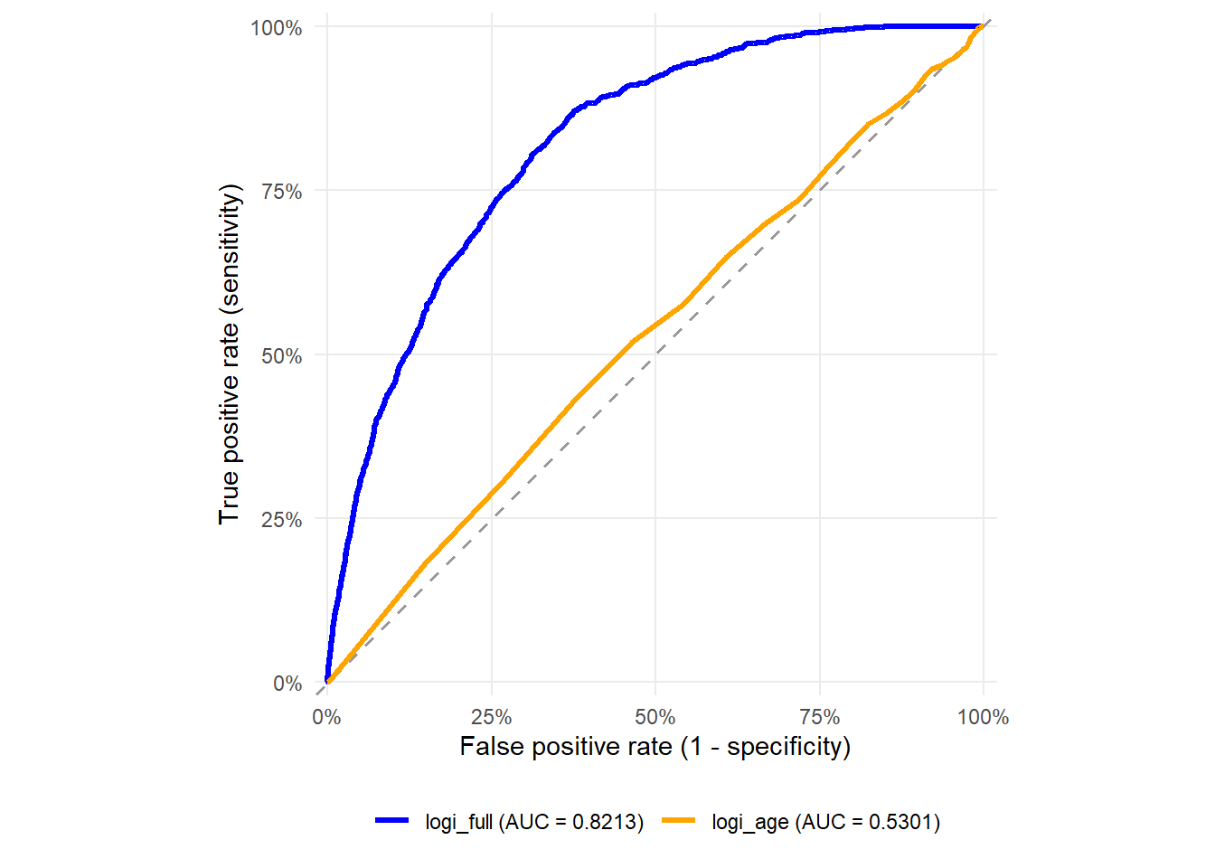
In Figure 1.16, the blue curve for logi_full dominates the orange curve for logi_age over most of the plot. This indicates that logi_full gives a better ranking of high-risk and low-risk applicants. The exact AUC values make that comparison explicit:
Code
      model    auc
1 logi_full 0.8213
2  logi_age 0.5301
The logi_age model has an AUC of 0.5301, which is close to the value produced by random ranking. That means age alone adds very little useful ranking information in this application. The logi_full model has an AUC of 0.8213, so it ranks defaulting applicants above non-defaulting applicants much more effectively.
AUC asks a ranking question. Do applicants who default tend to receive higher predicted probabilities than applicants who do not default? Calibration answers a probability question. If the model assigns a group of applicants an average predicted probability of default of 20%, do about 20% of those applicants actually default?
This distinction is important because we have been calling the output of the model a probability of default. If the model is well calibrated, the predicted probabilities can be interpreted more literally. If the model is poorly calibrated, the model may still be useful for ranking applicants from low risk to high risk, but the numerical probability values should be interpreted with more caution.
One simple way to inspect calibration is to divide the test set into groups according to the predicted probability of default. Here we use ten groups, or deciles. The first decile contains the applicants with the lowest predicted probabilities, and the tenth decile contains the applicants with the highest predicted probabilities. Then, for each decile and each model, we compare the average predicted probability with the observed default rate.
Code
calibration_data <- bind_rows(
  data.frame(
    model = "logi_full",
    observed_default = as.numeric(as.character(test$loan_st)),
    predicted_pd = pred_logi_full
  ),
  data.frame(
    model = "logi_age",
    observed_default = as.numeric(as.character(test$loan_st)),
    predicted_pd = pred_logi_age
  )
)

calibration_models <- calibration_data |>
  group_by(model) |>
  mutate(risk_decile = ntile(predicted_pd, 10)) |>
  group_by(model, risk_decile) |>
  summarize(
    applications = n(),
    average_predicted_pd = mean(predicted_pd),
    observed_default_rate = mean(observed_default),
    .groups = "drop"
  ) |>
  ungroup()

calibration_models |>
  mutate(
    average_predicted_pd = fmt_pct(average_predicted_pd, 2),
    observed_default_rate = fmt_pct(observed_default_rate, 2)
  ) |>
  knitr::kable(
    caption = "Calibration by predicted-risk decile for the full and age-only models.",
    row.names = FALSE
)| model | risk_decile | applications | average_predicted_pd | observed_default_rate |
|---|---|---|---|---|
| logi_age | 1 | 970 | 10.32% | 9.79% |
| logi_age | 2 | 970 | 10.81% | 9.59% |
| logi_age | 3 | 970 | 11.01% | 10.93% |
| logi_age | 4 | 970 | 11.14% | 9.79% |
| logi_age | 5 | 970 | 11.24% | 9.38% |
| logi_age | 6 | 969 | 11.32% | 10.22% |
| logi_age | 7 | 969 | 11.39% | 11.87% |
| logi_age | 8 | 969 | 11.45% | 12.18% |
| logi_age | 9 | 969 | 11.50% | 12.49% |
| logi_age | 10 | 969 | 11.55% | 13.11% |
| logi_full | 1 | 970 | 0.00% | 0.00% |
| logi_full | 2 | 970 | 0.79% | 0.72% |
| logi_full | 3 | 970 | 1.89% | 2.06% |
| logi_full | 4 | 970 | 3.04% | 3.40% |
| logi_full | 5 | 970 | 4.85% | 4.33% |
| logi_full | 6 | 969 | 7.74% | 7.12% |
| logi_full | 7 | 969 | 12.22% | 12.90% |
| logi_full | 8 | 969 | 17.20% | 15.69% |
| logi_full | 9 | 969 | 23.78% | 23.01% |
| logi_full | 10 | 969 | 40.96% | 40.14% |
The interpretation is direct. If the average predicted probability and the observed default rate are close within each decile, the model is reasonably calibrated for that part of the risk distribution. If the observed default rate is systematically above the predicted probability, the model is underestimating credit risk. If the observed default rate is systematically below the predicted probability, the model is overestimating credit risk.
The same idea appears in the next plot. The dashed line represents perfect calibration. Points close to the dashed line indicate that predicted probabilities and observed default rates are similar. Points far from the dashed line indicate calibration problems. The colors match the ROC figure, with blue for the full model and orange for the age model.
Code
ggplot(calibration_models,
       aes(x = average_predicted_pd, y = observed_default_rate,
           color = model)) +
  geom_abline(intercept = 0, slope = 1, linetype = "dashed",
              color = "gray50") +
  geom_line(linewidth = 1) +
  geom_point(size = 3) +
  scale_color_manual(values = c("logi_full" = "blue", "logi_age" = "orange")) +
  scale_x_continuous(labels = scales::percent_format(accuracy = 1)) +
  scale_y_continuous(labels = scales::percent_format(accuracy = 1)) +
  labs(x = "Average predicted probability of default",
       y = "Observed default rate",
       color = "Model") +
  theme_minimal() +
  theme(legend.position = "bottom")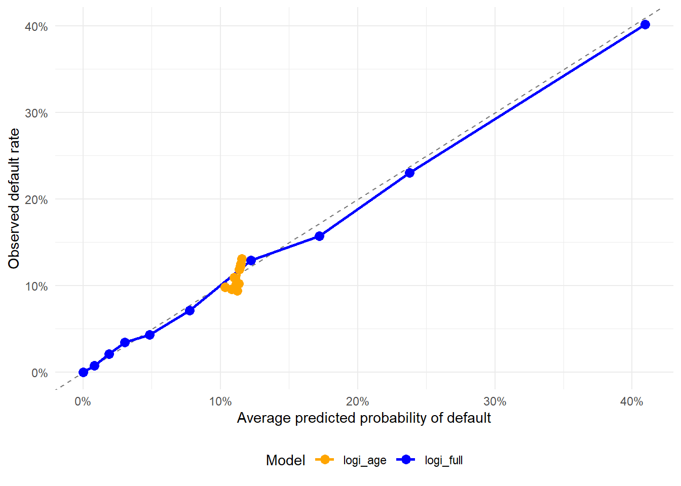
The Brier score gives us a compact numerical summary of probability prediction error. It is the average squared distance between the predicted probability and the observed outcome, where the observed outcome is 1 for default and 0 for no default:
\[ \text{Brier score} = \frac{1}{n}\sum_{i=1}^{n}(\hat{p}_i - y_i)^2. \]
A lower Brier score indicates better probability predictions. The measure is useful here because it evaluates the probabilities directly, before converting them into a binary accept/reject decision. The function brier_score(actual, predicted_probability) implements the formula directly. In that function, actual is \(y_i\), predicted_probability is \(\hat p_i\), and mean((predicted_probability - actual)^2) is the average squared error.
Code
brier_score <- function(actual, predicted_probability) {
  mean((predicted_probability - actual)^2)
}

actual_default <- as.numeric(as.character(test$loan_st))
constant_pd <- rep(mean(actual_default), length(actual_default))

brier_results <- data.frame(
  model = c("logi_full", "logi_age", "constant default rate"),
  brier_score = c(
    brier_score(actual_default, pred_logi_full),
    brier_score(actual_default, pred_logi_age),
    brier_score(actual_default, constant_pd)
  )
)

baseline_brier <- brier_results$brier_score[
  brier_results$model == "constant default rate"
]
brier_results$brier_skill <- 1 - brier_results$brier_score / baseline_brier

brier_results |>
  mutate(
    brier_score = fmt_num(brier_score, 4),
    brier_skill = fmt_num(brier_skill, 4)
  ) |>
  knitr::kable(
    caption = "Brier score and Brier skill against a constant default-rate benchmark.",
    row.names = FALSE
)| model | brier_score | brier_skill |
|---|---|---|
| logi_full | 0.0822 | 0.1559 |
| logi_age | 0.0973 | 0.0004 |
| constant default rate | 0.0974 | 0.0000 |
The constant default-rate model is a simple benchmark. It assigns the same probability of default to every applicant, equal to the observed default rate in the test set. A useful probability model should improve on that benchmark. The Brier skill score expresses this improvement relative to the benchmark.
\[ \text{Brier skill} = 1 - \frac{\text{Brier score of the model}} {\text{Brier score of the benchmark}}. \]
A value close to 0 means the model is barely improving on the constant default-rate benchmark; a positive value means the model reduces probability error relative to that benchmark. In code, baseline_brier is the denominator and 1 - brier_results$brier_score / baseline_brier is the Brier skill calculation. The Brier score combines probability accuracy with the model’s ability to separate high-risk and low-risk applicants, so it is a convenient way to summarize whether the predicted probabilities are numerically close to the observed default outcomes.
In practice, discrimination and calibration answer complementary questions. AUC helps us decide whether the model ranks applicants in a useful way. Calibration helps us decide whether the estimated probabilities can be interpreted as realistic probabilities of default. A lending strategy can benefit from both. Ranking is useful for deciding whom to accept or reject, while calibration is useful for pricing, provisioning, stress testing, and communicating the meaning of a predicted probability.
We can now return to the business rule. A cutoff converts a predicted probability into an accept/reject decision. Under our convention, a higher sensitivity means fewer defaulting borrowers are mistakenly accepted. A higher specificity means fewer good borrowers are mistakenly rejected.
The trade-off is financial. A very low cutoff rejects many applicants and tends to increase sensitivity, but it can reject many good borrowers. A very high cutoff accepts more applicants and tends to increase specificity, but it can accept more borrowers who default. The right balance depends on risk appetite, profitability, and regulation.
The two extreme policies make the problem clear. Accepting everyone maximizes loan volume and also accepts every default. Rejecting everyone eliminates accepted defaults and issues no loans. Useful credit policy lives between those extremes.
We evaluate two lending policies reviewed before. In the first policy, the bank wants to accept about 80% of applications. In the second policy, the bank wants to accept about 65%. This policy target is chosen before looking at the final classification counts.
The model then converts each policy into a probability cutoff. In R, this is done with quantile(). The call quantile(pred_logi_full, probs = 0.80) returns the empirical 80th percentile of the full model’s predicted default probabilities. We use that value as the cutoff because it places about 80% of the predicted probabilities at or below the cutoff. Those applications are accepted. Applications above the cutoff are rejected because their predicted default probabilities are in the riskiest part of the test set. The same logic gives the 65% policy by using probs = 0.65.
The word about is important. The bank chooses the policy target first, such as accepting about 80% of applications. Then quantile() finds an empirical cutoff from the ordered predicted probabilities. In R, the default quantile calculation may interpolate between adjacent ordered predictions. It does not smooth the whole distribution; it produces one cutoff value from the sample. After that, the accept/reject rule is applied to the observed predictions. If predicted probabilities are spread smoothly with few ties near the cutoff, the realized acceptance rate will be very close to the policy target. If many predictions are tied or tightly clustered around the cutoff, the realized rate can move a little farther from the target. In our code, applications with predicted default probability at or below the cutoff are accepted, while applications above the cutoff are rejected.
Code
# Calculate sensitivity and specificity from a confusion matrix.
classification_metrics <- function(actual, predicted) {
  cm <- table(
    Actual = factor(actual, levels = c("0", "1")),
    Predicted = factor(predicted, levels = c(0, 1))
  )
  tn <- cm["0", "0"]
  fp <- cm["0", "1"]
  fn <- cm["1", "0"]
  tp <- cm["1", "1"]
  c(
    sensitivity = as.numeric(tp / (tp + fn)),
    specificity = as.numeric(tn / (tn + fp))
  )
}

# Cutoffs implied by target acceptance rates.
cutoff_full_80 <- unname(quantile(pred_logi_full, probs = 0.80))
cutoff_age_80 <- unname(quantile(pred_logi_age, probs = 0.80))
cutoff_full_65 <- unname(quantile(pred_logi_full, probs = 0.65))
cutoff_age_65 <- unname(quantile(pred_logi_age, probs = 0.65))

# Binary predictions: 1 = reject as predicted default, 0 = accept.
pred_full_80 <- ifelse(pred_logi_full > cutoff_full_80, 1, 0)
pred_age_80 <- ifelse(pred_logi_age > cutoff_age_80, 1, 0)
pred_full_65 <- ifelse(pred_logi_full > cutoff_full_65, 1, 0)
pred_age_65 <- ifelse(pred_logi_age > cutoff_age_65, 1, 0)

metrics_full_80 <- classification_metrics(test$loan_st, pred_full_80)
metrics_age_80 <- classification_metrics(test$loan_st, pred_age_80)
metrics_full_65 <- classification_metrics(test$loan_st, pred_full_65)
metrics_age_65 <- classification_metrics(test$loan_st, pred_age_65)

# Combine the results.
results_df <- data.frame(
  Model = c("logi_full", "logi_age", "logi_full", "logi_age"),
  Policy = c("Accept about 80%", "Accept about 80%",
             "Accept about 65%", "Accept about 65%"),
  Accepted_in_test_set = c(mean(pred_full_80 == 0),
                           mean(pred_age_80 == 0),
                           mean(pred_full_65 == 0),
                           mean(pred_age_65 == 0)),
  PD_cutoff = c(cutoff_full_80, cutoff_age_80,
                cutoff_full_65, cutoff_age_65),
  Sensitivity = c(metrics_full_80["sensitivity"],
                  metrics_age_80["sensitivity"],
                  metrics_full_65["sensitivity"],
                  metrics_age_65["sensitivity"]),
  Specificity = c(metrics_full_80["specificity"],
                  metrics_age_80["specificity"],
                  metrics_full_65["specificity"],
                  metrics_age_65["specificity"])
)

results_df |>
  mutate(
    Accepted_in_test_set = fmt_pct(Accepted_in_test_set, 1),
    PD_cutoff = fmt_pct(PD_cutoff, 2),
    Sensitivity = fmt_pct(Sensitivity, 1),
    Specificity = fmt_pct(Specificity, 1)
  ) |>
  knitr::kable(
    caption = "Cutoffs and error rates implied by two acceptance policies.",
    col.names = c(
      "Model",
      "Bank policy",
      "Accepted in test set",
      "PD cutoff",
      "Sensitivity",
      "Specificity"
    ),
    row.names = FALSE
)| Model | Bank policy | Accepted in test set | PD cutoff | Sensitivity | Specificity |
|---|---|---|---|---|---|
| logi_full | Accept about 80% | 80.0% | 19.95% | 57.8% | 84.6% |
| logi_age | Accept about 80% | 85.0% | 11.46% | 18.0% | 85.4% |
| logi_full | Accept about 65% | 65.0% | 12.23% | 77.9% | 70.3% |
| logi_age | Accept about 65% | 72.6% | 11.40% | 30.9% | 73.1% |
The summary table should be read as a policy comparison. Policy is the acceptance goal chosen by the bank. PD_cutoff is the predicted default probability that implements that goal. Accepted_in_test_set is the share of applications actually accepted after applying the cutoff. Moving from the 80% policy to the 65% policy makes the rule more conservative because more applicants are rejected. That change usually detects more actual defaults, raising sensitivity. It also rejects more non-defaulting applicants, reducing specificity.
Code
roc_full_df <- roc_to_df_logistic(ROC_logi_full, "logi_full") |>
  arrange(false_positive_rate)

roc_acceptance_guides <- data.frame(
  target = c("Acceptance rate of 80%", "Acceptance rate of 65%"),
  false_positive_rate = c(
    1 - metrics_full_80["specificity"],
    1 - metrics_full_65["specificity"]
  ),
  true_positive_rate = c(
    metrics_full_80["sensitivity"],
    metrics_full_65["sensitivity"]
  )
)

roc_acceptance_labels <- data.frame(
  target = c("Acceptance rate of 80%", "Acceptance rate of 65%"),
  false_positive_rate = roc_acceptance_guides$false_positive_rate,
  true_positive_rate = roc_acceptance_guides$true_positive_rate,
  label_x = c(0.56, 0.56),
  label_y = c(0.55, 0.84),
  label = c(
    paste0(
      "80% policy\n",
      "Sensitivity = ", fmt_pct(metrics_full_80["sensitivity"], 1), "\n",
      "Specificity = ", fmt_pct(metrics_full_80["specificity"], 1)
    ),
    paste0(
      "65% policy\n",
      "Sensitivity = ", fmt_pct(metrics_full_65["sensitivity"], 1), "\n",
      "Specificity = ", fmt_pct(metrics_full_65["specificity"], 1)
    )
  )
)

ggplot(roc_full_df, aes(x = false_positive_rate, y = true_positive_rate)) +
  geom_abline(
    intercept = 0,
    slope = 1,
    linetype = "dashed",
    color = "gray60",
    linewidth = 0.7
  ) +
  geom_line(color = "blue", linewidth = 1.2) +
  geom_segment(
    data = roc_acceptance_guides,
    aes(
      x = false_positive_rate,
      xend = false_positive_rate,
      y = 0,
      yend = true_positive_rate,
      color = target
    ),
    inherit.aes = FALSE,
    linetype = "dashed",
    linewidth = 1
  ) +
  geom_segment(
    data = roc_acceptance_guides,
    aes(
      x = 0,
      xend = false_positive_rate,
      y = true_positive_rate,
      yend = true_positive_rate,
      color = target
    ),
    inherit.aes = FALSE,
    linetype = "dashed",
    linewidth = 1
  ) +
  geom_point(
    data = roc_acceptance_guides,
    aes(
      x = false_positive_rate,
      y = true_positive_rate,
      color = target
    ),
    inherit.aes = FALSE,
    size = 2.8
  ) +
  geom_segment(
    data = roc_acceptance_labels,
    aes(
      x = false_positive_rate,
      xend = label_x - 0.02,
      y = true_positive_rate,
      yend = label_y,
      color = target
    ),
    inherit.aes = FALSE,
    linewidth = 0.45,
    alpha = 0.7,
    show.legend = FALSE
  ) +
  geom_label(
    data = roc_acceptance_labels,
    aes(
      x = label_x,
      y = label_y,
      label = label,
      color = target
    ),
    inherit.aes = FALSE,
    hjust = 0,
    size = 3.1,
    lineheight = 0.95,
    label.size = 0.25,
    label.padding = grid::unit(0.15, "lines"),
    fill = "white",
    show.legend = FALSE
  ) +
  scale_color_manual(
    values = c("Acceptance rate of 80%" = "red",
               "Acceptance rate of 65%" = "black"),
    name = NULL
  ) +
  scale_x_continuous(
    labels = scales::percent_format(accuracy = 1),
    limits = c(0, 1),
    expand = c(0.01, 0.01)
  ) +
  scale_y_continuous(
    labels = scales::percent_format(accuracy = 1),
    limits = c(0, 1),
    expand = c(0.01, 0.01)
  ) +
  labs(
    x = "False positive rate (1 - specificity)",
    y = "True positive rate (sensitivity)"
  ) +
  coord_equal() +
  theme_minimal() +
  theme(
    legend.position = "bottom",
    panel.grid.minor = element_blank()
  )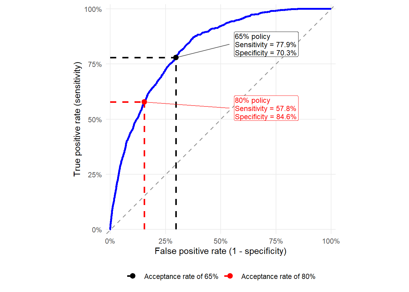
Figure 1.18 places the two full-model policies on the same ROC curve. The red point corresponds to the 80% acceptance rule, which rejects only the riskiest 20% of applicants. The black point corresponds to the 65% acceptance rule, which rejects the riskiest 35%. The black point is higher because the stricter rule catches more actual defaults. It is also farther to the right because the stricter rule rejects more applicants who would not have defaulted. The figure therefore turns the cutoff choice into a visible risk-management trade-off.
The next two confusion-matrix outputs verify the same logic numerically. Rows are actual outcomes. Columns are lending decisions implied by the model. Accept means predicted no-default and Reject means predicted default.
For the 80% acceptance target:
Code
cm_full_80 <- table(
  Actual = factor(
    test$loan_st,
    levels = c("0", "1"),
    labels = c("No default", "Default")
  ),
  Decision = factor(
    pred_full_80,
    levels = c(0, 1),
    labels = c("Accept", "Reject")
  )
)
tn_80 <- cm_full_80["No default", "Accept"]
fp_80 <- cm_full_80["No default", "Reject"]
fn_80 <- cm_full_80["Default", "Accept"]
tp_80 <- cm_full_80["Default", "Reject"]
sens_80 <- as.numeric(tp_80 / (tp_80 + fn_80))
spec_80 <- as.numeric(tn_80 / (tn_80 + fp_80))

cm_full_80
Decision
Actual Accept Reject
No default 7309 1326
Default 447 613For this rule, the model rejects 613 applicants who actually default and accepts 447 applicants who later default. Sensitivity is therefore 0.5783. The model accepts 7309 applicants who do not default and rejects 1326 applicants who do not default. Specificity is therefore 0.8464.
For the 65% acceptance target:
Code
cm_full_65 <- table(
  Actual = factor(
    test$loan_st,
    levels = c("0", "1"),
    labels = c("No default", "Default")
  ),
  Decision = factor(
    pred_full_65,
    levels = c(0, 1),
    labels = c("Accept", "Reject")
  )
)
tn_65 <- cm_full_65["No default", "Accept"]
fp_65 <- cm_full_65["No default", "Reject"]
fn_65 <- cm_full_65["Default", "Accept"]
tp_65 <- cm_full_65["Default", "Reject"]
sens_65 <- as.numeric(tp_65 / (tp_65 + fn_65))
spec_65 <- as.numeric(tn_65 / (tn_65 + fp_65))

cm_full_65
Decision
Actual Accept Reject
No default 6068 2567
Default 234 826For this rule, the model rejects 826 applicants who actually default and accepts 234 applicants who later default. Sensitivity rises to 0.7792. The cost is visible among non-defaulting applicants. The model accepts 6068 of them and rejects 2567 of them, so specificity falls to 0.7027.
The comparison shows why a cutoff is a business decision. The 65% acceptance rule protects the lender from more defaults, but it also turns away more borrowers who would have repaid. The 80% acceptance rule keeps more business volume and rejects fewer good borrowers, while allowing more defaulting borrowers into the portfolio.
A pure-random score would look like this:
Code
set.seed(2020)
pred_rand_model <- runif(length(pred_logi_age))
ROC_rand <- roc(test$loan_st, pred_rand_model, quiet = TRUE)
auc_rand <- as.numeric(auc(ROC_rand))

roc_rand_df <- roc_to_df_logistic(ROC_rand, "Random score") |>
  arrange(false_positive_rate)

ggplot(roc_rand_df, aes(x = false_positive_rate, y = true_positive_rate)) +
  geom_abline(
    intercept = 0,
    slope = 1,
    linetype = "dashed",
    color = "gray60",
    linewidth = 0.7
  ) +
  geom_line(color = "red", linewidth = 1.2) +
  scale_x_continuous(
    labels = scales::percent_format(accuracy = 1),
    limits = c(0, 1),
    expand = c(0.01, 0.01)
  ) +
  scale_y_continuous(
    labels = scales::percent_format(accuracy = 1),
    limits = c(0, 1),
    expand = c(0.01, 0.01)
  ) +
  labs(
    x = "False positive rate (1 - specificity)",
    y = "True positive rate (sensitivity)"
  ) +
  coord_equal() +
  theme_minimal() +
  theme(panel.grid.minor = element_blank())

c(random_score_auc = round(auc_rand, 4))
random_score_auc
0.5105 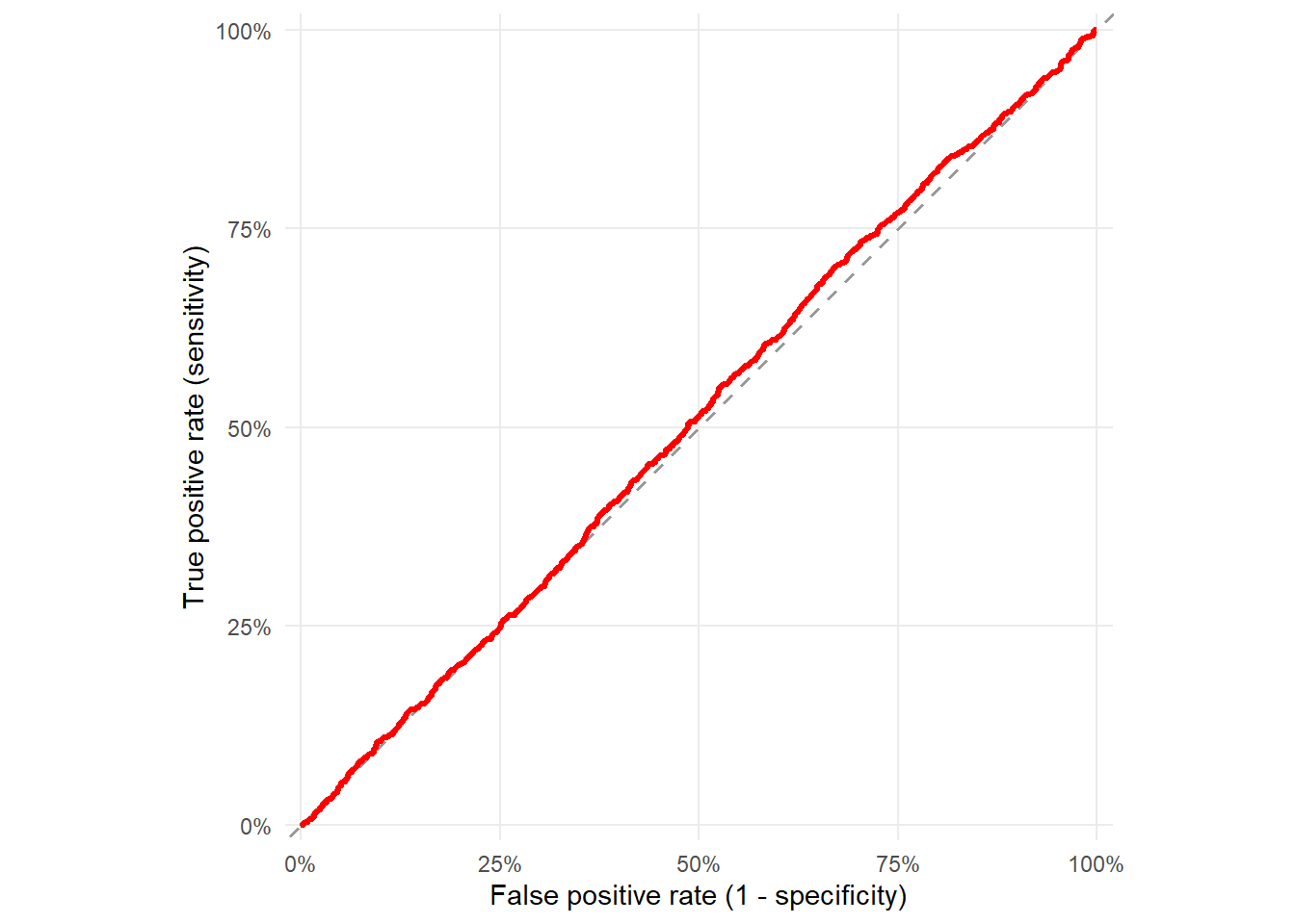
A random score should produce a ROC curve close to the diagonal. The area under that diagonal is 0.5, so an AUC close to 0.5 means the score has almost no ranking power. Because the code uses a finite random sample, the reported AUC can be close to 0.5 without being exactly 0.5.
A perfect score gives the opposite benchmark:
Code
pred_perfect_model <- as.numeric(as.character(test$loan_st))
ROC_perfect <- roc(test$loan_st, pred_perfect_model, quiet = TRUE)
auc_perfect <- as.numeric(auc(ROC_perfect))

roc_perfect_df <- data.frame(
  false_positive_rate = c(0, 0, 1),
  true_positive_rate = c(0, 1, 1)
)

ggplot(roc_perfect_df, aes(x = false_positive_rate, y = true_positive_rate)) +
  geom_abline(
    intercept = 0,
    slope = 1,
    linetype = "dashed",
    color = "gray60",
    linewidth = 0.7
  ) +
  geom_path(color = "blue", linewidth = 1.2) +
  scale_x_continuous(
    labels = scales::percent_format(accuracy = 1),
    limits = c(0, 1),
    expand = c(0.01, 0.01)
  ) +
  scale_y_continuous(
    labels = scales::percent_format(accuracy = 1),
    limits = c(0, 1.02),
    breaks = seq(0, 1, 0.25),
    expand = c(0.01, 0.01)
  ) +
  labs(
    x = "False positive rate (1 - specificity)",
    y = "True positive rate (sensitivity)"
  ) +
  coord_equal() +
  theme_minimal() +
  theme(panel.grid.minor = element_blank())

c(perfect_score_auc = round(auc_perfect, 4))
perfect_score_auc
1 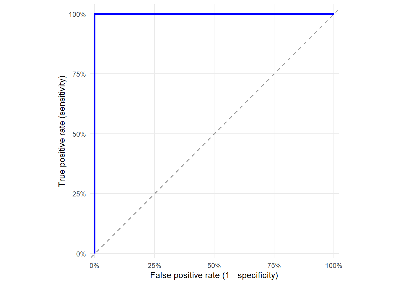
In a perfect score, every applicant who defaults receives a higher score than every applicant who does not default. The ROC curve therefore rises vertically from 0% to 100% sensitivity while the false positive rate is still 0%, and then moves horizontally along the top of the graph. The AUC is 1. At the right cutoff, the model identifies all defaults and all non-defaults correctly, giving 100% sensitivity and 100% specificity.
1.8 What do we gain and what do we lose?
Logistic regression gives us a transparent credit-scoring benchmark. The model produces a predicted probability of default, and the coefficients can be interpreted through log-odds and odds ratios. This makes the model easier to audit, explain, and connect to a lending rule.
The cost of that transparency is structure. Unless we manually add nonlinear terms or interactions, the model assumes a relatively simple relationship between the predictors and the log-odds of default. That can be too restrictive if credit risk depends on combinations of variables, such as interest rate and grade, or loan amount and income.
The main gain from this chapter is therefore a disciplined workflow. We started with a probability model, converted probabilities into cutoff decisions, evaluated the resulting accepted portfolio, and connected the cutoff to bad rates, calibration, AUC, Brier score, and net payoff. The next chapter keeps the same credit scoring problem and the same evaluation logic, but changes the model class. That lets us ask a sharper question. Can tree-based models capture interactions and nonlinear patterns that the logistic benchmark may miss, and do those extra patterns improve credit decisions out of sample?