6 Climate Credit Risk

Climate credit risk asks how climate-related shocks can change the default risk of borrowers, the expected loss of a loan portfolio, and the compensation required in credit markets. The credit-risk object is familiar from the previous chapters. We still work with probability of default, exposure at default, loss given default, expected loss, credit spreads, and portfolio loss distributions. The new element is the source of the shock.

A climate shock can reach credit risk through two channels. Transition risk comes from policy, technology, energy prices, consumer demand, and the speed of decarbonization. Physical risk comes from acute events such as floods, heatwaves, droughts, storms, and wildfires, and from chronic changes that affect production, infrastructure, insurance costs, and collateral values. The credit analyst’s task is to translate those channels into credit quantities that can be priced, provisioned, limited, or stress tested.

This chapter answers two practical questions.

How much credit risk is underestimated if climate risk is ignored?

Which sectors contribute most to climate credit risk?

The chapter uses public NGFS short-term climate scenario data. The Network for Greening the Financial System provides short-term climate scenarios for central banks and supervisors, and the scenario explorer is hosted by IIASA (Network for Greening the Financial System 2025; Network for Greening the Financial System and IIASA 2025). We use the CLIMACRED model inside that database because it reports financial credit-risk variables directly: baseline corporate probabilities of default, PD adjustments, corporate bond spread adjustments, corporate bond price adjustments, and WACC adjustments. Those variables let us keep the chapter applied. The climate-to-credit mapping is already supplied by the scenario database, so the chapter can focus on valuation, expected loss, sector contribution, and portfolio risk.

The regulatory motivation is also direct. The Basel Committee describes climate-related financial risks as drivers that can transmit into traditional risk types, including credit risk (Basel Committee on Banking Supervision 2021). Its principles for climate-related financial risk management ask banks and supervisors to identify, measure, monitor, and control those risks (Basel Committee on Banking Supervision 2022). EBA guidelines require institutions to integrate environmental, social, and governance risks into risk-management frameworks (European Banking Authority 2025b). The EBA guidelines on environmental scenario analysis are especially relevant here because they specify supervisory expectations for forward-looking environmental scenario analysis, stress testing, and resilience analysis (European Banking Authority 2025a). IFRS S2 focuses disclosure on climate-related risks and opportunities that can affect cash flows, access to finance, and cost of capital (IFRS Foundation 2023). For our purposes, that means the modeling object should look like something a bank, investor, or risk analyst can actually use.

This is why climate credit risk belongs in a credit-risk book. A credit committee needs to ask whether a borrower becomes riskier when energy prices, carbon policy, technology, weather damage, insurance costs, or collateral values change. A risk-management function needs a way to translate that question into PDs, LGDs, spreads, prices, limits, provisions, stress-test losses, and portfolio concentrations. A disclosure team needs a coherent explanation of how climate-related risks can affect financing costs and future cash flows. The chapter turns those institutional needs into a reproducible workflow.

The route through the chapter is sequential. First, we define the data source and explain the scenario objects. Second, we build a global sector loan portfolio with USD 100 million of exposure. Third, we download CLIMACRED data and clean it into a credit-risk table. Fourth, we convert scenario PDs into expected loss over a five-year horizon. Fifth, we identify the sectors responsible for the incremental expected loss. Sixth, we connect the same climate credit quantities to spreads, bond prices, and CDS-style compensation. Finally, we run a simple portfolio loss simulation to show how climate-adjusted PDs change the loss distribution.

6.1 From climate scenarios to credit quantities

A climate scenario is a structured state of the world used for risk analysis. In this chapter, the scenario tells us how sector-level credit variables change over time under a particular climate narrative. The credit-risk calculations then ask what those changes do to a portfolio.

The important separation is this.

The external data come from NGFS/IIASA. The bank portfolio is a teaching portfolio that we define inside the chapter. In real work, the bank would replace our exposure and recovery inputs with its own loan book. The NGFS data would still enter as the scenario layer.

The scenario layer should be read as a credit overlay. Suppose a bank lends to a coal producer, a power utility, an airline, and a technology hardware firm. The bank already has a baseline view of credit quality. Climate analysis asks how that baseline changes if the economy follows a particular transition or physical-risk path. The model focuses on sector-level credit adjustments that can be connected to the same instruments the bank already manages: loans, bonds, CDS, and portfolio limits.

The NGFS short-term database gives several scenario runs. The names below are official NGFS short-term scenario narratives in the IIASA Scenario Explorer, not labels created for this chapter. We use three global CLIMACRED runs for the main portfolio analysis. The scenario code is the short name used in our cleaned data, and the run ID is the numerical identifier used by the API request.

Code

scenario_table <- data.frame(
  `Scenario code` = c("DIRE", "HWTP", "SWUC"),
  `NGFS scenario narrative` = c(
    "Diverging Realities",
    "Highway to Paris",
    "Sudden Wake-up Call"
  ),
  `API run ID` = c(74, 75, 76),
  `Main credit-risk channel` = c(
    "Mixed transition and physical pressure",
    "Orderly but demanding transition pressure",
    "Delayed transition shock"
  ),
  `Reading in this chapter` = c(
    "Climate policy and climate damage are uneven across regions and sectors.",
    "The transition is more coordinated, but high-emission sectors still face credit stress.",
    "The market reprices climate risk abruptly after a period of limited adjustment."
  ),
  check.names = FALSE
)

kable(
  scenario_table,
  row.names = FALSE,
  caption = "Global NGFS short-term CLIMACRED scenarios used in the main analysis."
)

Global NGFS short-term CLIMACRED scenarios used in the main analysis.
Scenario code	NGFS scenario narrative	API run ID	Main credit-risk channel	Reading in this chapter
DIRE	Diverging Realities	74	Mixed transition and physical pressure	Climate policy and climate damage are uneven across regions and sectors.
HWTP	Highway to Paris	75	Orderly but demanding transition pressure	The transition is more coordinated, but high-emission sectors still face credit stress.
SWUC	Sudden Wake-up Call	76	Delayed transition shock	The market reprices climate risk abruptly after a period of limited adjustment.

We also use the regional DAPS runs to keep physical risk visible. Those runs are useful because physical shocks are naturally local. A flood, heatwave, storm, or drought affects some regions more than others. For that reason, the main portfolio analysis uses the global World region, while the physical-risk check uses the regional DAPS runs.

Code

climate_channel_map <- data.frame(
  Channel = c(
    "Transition risk",
    "Physical risk"
  ),
  `Typical credit mechanism` = c(
    "Policy, technology, energy prices, demand, and cost-of-capital changes affect sector cash flows and refinancing capacity.",
    "Flood, heat, drought, storm, wildfire, and chronic climate stress affect assets, operations, collateral, insurance costs, and supply chains."
  ),
  `How this chapter uses it` = c(
    "The main portfolio workflow uses global CLIMACRED scenario adjustments by sector.",
    "The DAPS block is a regional diagnostic that shows why a full physical-risk credit model needs location."
  ),
  `Data needed for a production model` = c(
    "Borrower sector, exposure, maturity, recovery, baseline credit quality, and scenario mapping.",
    "Borrower and collateral geography, hazard intensity, vulnerability, insurance, business interruption, and supply-chain exposure."
  ),
  check.names = FALSE
)

kable(
  climate_channel_map,
  caption = "How transition and physical climate risk enter credit analysis in this chapter.",
  row.names = FALSE
)

How transition and physical climate risk enter credit analysis in this chapter.
Channel	Typical credit mechanism	How this chapter uses it	Data needed for a production model
Transition risk	Policy, technology, energy prices, demand, and cost-of-capital changes affect sector cash flows and refinancing capacity.	The main portfolio workflow uses global CLIMACRED scenario adjustments by sector.	Borrower sector, exposure, maturity, recovery, baseline credit quality, and scenario mapping.
Physical risk	Flood, heat, drought, storm, wildfire, and chronic climate stress affect assets, operations, collateral, insurance costs, and supply chains.	The DAPS block is a regional diagnostic that shows why a full physical-risk credit model needs location.	Borrower and collateral geography, hazard intensity, vulnerability, insurance, business interruption, and supply-chain exposure.

Each scenario row should therefore be read as a different question for risk management. Diverging Realities asks what happens when the adjustment is uneven. Highway to Paris asks what an orderly but demanding transition does to sector credit risk. Sudden Wake-up Call asks what happens when markets and policy adjust after delay. These are scenario narratives from the NGFS database (Network for Greening the Financial System 2025; Network for Greening the Financial System and IIASA 2025). Our contribution is to translate the CLIMACRED credit outputs from those runs into PDs, expected losses, spreads, bond-price effects, and portfolio loss simulations.

The CLIMACRED variables we need are:

Code

ngfs_variable_table <- data.frame(
  variable = c(
    "baseline_pd",
    "pd_adjustment",
    "corporate_bond_spread_adjustment",
    "corporate_bond_price_rel_adjustment",
    "wacc_adjustment"
  ),
  unit = c(
    "Percentage points",
    "Percentage points relative to BAU",
    "Percentage points relative to BAU",
    "Percent relative to BAU",
    "Percentage points relative to BAU"
  ),
  role = c(
    "Default risk before the climate adjustment.",
    "Climate-related change in sector PD.",
    "Credit-spread change implied by the scenario.",
    "Corporate bond price change implied by the scenario.",
    "Cost-of-capital change implied by the scenario."
  )
)

kable(
  ngfs_variable_table,
  caption = "CLIMACRED variables used in the chapter."
)

CLIMACRED variables used in the chapter.
variable	unit	role
baseline_pd	Percentage points	Default risk before the climate adjustment.
pd_adjustment	Percentage points relative to BAU	Climate-related change in sector PD.
corporate_bond_spread_adjustment	Percentage points relative to BAU	Credit-spread change implied by the scenario.
corporate_bond_price_rel_adjustment	Percent relative to BAU	Corporate bond price change implied by the scenario.
wacc_adjustment	Percentage points relative to BAU	Cost-of-capital change implied by the scenario.

The table also explains why CLIMACRED is useful pedagogically. baseline_pd gives the ordinary credit-risk starting point. pd_adjustment is the climate overlay. The spread and price adjustments connect the credit shock to traded credit instruments. The WACC adjustment reminds us that climate risk can also affect the cost of capital, which feeds into investment, refinancing, and firm value. The chapter uses these variables with different intensity, and showing them together helps students see the full credit-market chain.

Read pd_adjustment carefully. If the baseline PD is 4.00 percentage points and the climate PD adjustment is 1.50 percentage points, the climate-stressed PD is 5.50 percentage points. In decimal notation:

\[ PD^{climate}_{i,t,s} = \min\left( PD^{base}_{i,t,s}+\Delta PD^{climate}_{i,t,s}, 1 \right). \]

The subscript $i$ denotes the sector, $t$ the year, and $s$ the scenario. The operator $\min$ caps the stressed PD at 100%. Most observations in this chapter are far below that cap, but the formula keeps the transformation well defined.

6.2 Downloading NGFS data

The book uses a raw local copy of the NGFS/IIASA download. This is a reproducibility choice. A fixed input file makes the render stable, while the download script keeps the source transparent. The raw files used here are in data/raw, and they were created by R/download-ngfs-climate-credit-data.R.

The download itself is still part of the learning material. The script first obtains a guest token from the IIASA manager endpoint. Then it sends a JSON query to the CLIMACRED time-series endpoint. The important lesson is that the API request is explicit: we tell the database which runs, regions, variables, years, and time slice we want.

Code

ngfs_database <- "IXSE_NGFS_PHASE_5_SHORT_TERM"
ngfs_auth_url <- "https://api.manager.ece.iiasa.ac.at/legacy"
ngfs_base_url <- "https://db1.ene.iiasa.ac.at/ngfs-phase-5-short-term-api/rest/v2.1"

ngfs_get_guest_token <- function(max_tries = 5, wait_seconds = 1) {
  token_url <- paste0(ngfs_auth_url, "/anonym/", ngfs_database)

  for (try_id in seq_len(max_tries)) {
    response <- try(
      httr::GET(
        token_url,
        query = list(algorithm = "HS256"),
        httr::timeout(30)
      ),
      silent = TRUE
    )

    if (!inherits(response, "try-error") &&
        httr::status_code(response) == 200) {
      token <- httr::content(response, as = "text", encoding = "UTF-8")
      token <- gsub('^"|"$', "", token)

      if (nzchar(token)) {
        return(token)
      }
    }

    Sys.sleep(wait_seconds)
  }

  stop("The NGFS guest token could not be obtained. Check the internet connection or the NGFS/IIASA service.")
}

ngfs_post_timeseries <- function(runs, regions, variables, years = integer()) {
  token <- ngfs_get_guest_token()

  request_body <- list(
    filters = list(
      runs = as.list(as.integer(runs)),
      regions = as.list(regions),
      variables = as.list(variables),
      units = list(),
      years = as.list(as.integer(years)),
      timeslices = list("Year")
    )
  )

  response <- httr::POST(
    paste0(ngfs_base_url, "/runs/bulk/ts"),
    httr::add_headers(Authorization = paste("Bearer", token)),
    httr::content_type_json(),
    body = jsonlite::toJSON(request_body, auto_unbox = TRUE),
    encode = "raw",
    httr::timeout(120)
  )

  response_text <- httr::content(response, as = "text", encoding = "UTF-8")

  if (httr::status_code(response) != 200) {
    stop(response_text)
  }

  data <- jsonlite::fromJSON(response_text, flatten = TRUE)

  if (length(data) == 0) {
    stop("The NGFS query returned no observations. Check run names, regions, variables, or years.")
  }

  tibble::as_tibble(data)
}

The complete script also writes the raw responses to CSV files. A student who wants to refresh the data can run:

Code

source("R/download-ngfs-climate-credit-data.R")

The query uses the same field names students see in the scenario explorer: model, scenario, region, variable, year, and value. This keeps the data-cleaning step visible. In the chapter itself, we start from the raw CSV files created by the script. The objects below document the global request used by the downloader.

Code

global_runs <- c(
  "Diverging Realities" = 74,
  "Highway to Paris" = 75,
  "Sudden Wake-up Call" = 76
)

portfolio <- tibble::tibble(
  portfolio_sector = c(
    "Coal",
    "Oil",
    "Gas",
    "Power",
    "Land transport",
    "Air transport",
    "Construction",
    "Agriculture",
    "Chemicals",
    "Technology hardware"
  ),
  ngfs_sector = c(
    "Coal",
    "Oil",
    "Gas",
    "Power Supply",
    "Land transport",
    "Air transport",
    "Construction",
    "Agriculture",
    "Chemical Products",
    "Computer, electronic and optical products"
  ),
  ead = c(10, 12, 10, 12, 10, 8, 10, 8, 10, 10) * 1e6,
  recovery = c(0.35, 0.40, 0.42, 0.45, 0.40, 0.35, 0.45, 0.35, 0.42, 0.50)
)

metric_names <- c(
  "baseline_pd",
  "pd_adjustment",
  "corporate_bond_spread_adjustment",
  "corporate_bond_price_rel_adjustment",
  "wacc_adjustment"
)

ngfs_variables <- as.vector(
  outer(metric_names, portfolio$ngfs_sector, paste, sep = "|")
)

horizon_years <- 2026:2030

The portfolio totals USD 100 million. The exposures and recoveries are analyst inputs. They represent the bank’s own book. The external scenario data enter through the sector PD, spread, price, and WACC variables.

This separation is important for interpretation. The NGFS data do not describe this bank’s portfolio. They describe scenario credit shocks by sector, region, year, and variable. The portfolio table below is the bank-side input that tells the model where the money is exposed. The chapter combines the two layers only after both have been made explicit.

Code

portfolio_table <- portfolio |>
  mutate(
    EAD = fmt_usd_m(ead),
    Recovery = fmt_pct(recovery, 1),
    LGD = fmt_pct(1 - recovery, 1)
  ) |>
  transmute(
    `Portfolio sector` = portfolio_sector,
    `NGFS sector` = ngfs_sector,
    EAD,
    Recovery,
    LGD
  )

kable(
  portfolio_table,
  caption = "Teaching portfolio used for the climate credit-risk application."
)

Teaching portfolio used for the climate credit-risk application.
Portfolio sector	NGFS sector	EAD	Recovery	LGD
Coal	Coal	$10.00m	35.0%	65.0%
Oil	Oil	$12.00m	40.0%	60.0%
Gas	Gas	$10.00m	42.0%	58.0%
Power	Power Supply	$12.00m	45.0%	55.0%
Land transport	Land transport	$10.00m	40.0%	60.0%
Air transport	Air transport	$8.00m	35.0%	65.0%
Construction	Construction	$10.00m	45.0%	55.0%
Agriculture	Agriculture	$8.00m	35.0%	65.0%
Chemicals	Chemical Products	$10.00m	42.0%	58.0%
Technology hardware	Computer, electronic and optical products	$10.00m	50.0%	50.0%

The local files are a frozen copy of the API responses. They are raw in the practical sense needed for this chapter: the observations still have the original scenario code, region, variable string, unit, year, and value. The financial work begins in the next step, where we separate metrics from sectors, join the portfolio, convert percentage points into decimal PDs, and compute expected loss.

Code

ngfs_manifest <- utils::read.csv(
  file.path("data", "raw", "ngfs_climacred_download_manifest.csv"),
  stringsAsFactors = FALSE
)

ngfs_raw <- utils::read.csv(
  file.path("data", "raw", "ngfs_climacred_global_raw.csv"),
  stringsAsFactors = FALSE
)

ngfs_manifest |>
  transmute(
    File = file,
    Rows = rows,
    Database = database,
    `Downloaded at UTC` = downloaded_at_utc
  ) |>
  kable(caption = "Raw NGFS/IIASA files used in the chapter.")

Raw NGFS/IIASA files used in the chapter.
File	Rows	Database	Downloaded at UTC
data/raw/ngfs_climacred_global_raw.csv	1350	IXSE_NGFS_PHASE_5_SHORT_TERM	2026-06-04 03:31:44 UTC
data/raw/ngfs_climacred_daps_raw.csv	126	IXSE_NGFS_PHASE_5_SHORT_TERM	2026-06-04 03:31:44 UTC

Code

ngfs_raw |>
  select(model, scenario, region, variable, year, value) |>
  head(8) |>
  kable(caption = "First rows of the raw global CLIMACRED file.")

First rows of the raw global CLIMACRED file.
model	scenario	region	variable	year	value
CLIMACRED	DIRE	World	pd_adjustment\|Gas	2022	0.000000
CLIMACRED	DIRE	World	pd_adjustment\|Gas	2023	0.000000
CLIMACRED	DIRE	World	pd_adjustment\|Gas	2024	1.916841
CLIMACRED	DIRE	World	pd_adjustment\|Gas	2025	2.968586
CLIMACRED	DIRE	World	pd_adjustment\|Gas	2026	4.182788
CLIMACRED	DIRE	World	pd_adjustment\|Gas	2027	6.493470
CLIMACRED	DIRE	World	pd_adjustment\|Gas	2028	9.075679
CLIMACRED	DIRE	World	pd_adjustment\|Gas	2029	8.517978

Code

climate_data_provenance <- data.frame(
  Layer = c(
    "External scenario source",
    "Download script",
    "Frozen raw files",
    "Portfolio assumptions",
    "Clean analysis table"
  ),
  Object = c(
    "NGFS Short-term Scenario Explorer / IIASA API",
    "`R/download-ngfs-climate-credit-data.R`",
    "`data/raw/ngfs_climacred_global_raw.csv` and `data/raw/ngfs_climacred_daps_raw.csv`",
    "`portfolio`",
    "`climate_credit`"
  ),
  Role = c(
    "Supplies sector-level climate-credit variables by scenario, region, year, and metric.",
    "Documents the API request and refreshes the raw CSV files when the data source is available.",
    "Keep the book render reproducible and preserve the original scenario code, variable string, unit, year, and value.",
    "Defines the teaching bank's EAD and recovery assumptions by sector.",
    "Joins scenario data to portfolio assumptions and converts percentage-point variables into decimal credit quantities."
  )
)

kable(
  climate_data_provenance,
  caption = "Data provenance for the climate credit-risk workflow.",
  escape = FALSE
)

Data provenance for the climate credit-risk workflow.
Layer	Object	Role
External scenario source	NGFS Short-term Scenario Explorer / IIASA API	Supplies sector-level climate-credit variables by scenario, region, year, and metric.
Download script	`R/download-ngfs-climate-credit-data.R`	Documents the API request and refreshes the raw CSV files when the data source is available.
Frozen raw files	`data/raw/ngfs_climacred_global_raw.csv` and `data/raw/ngfs_climacred_daps_raw.csv`	Keep the book render reproducible and preserve the original scenario code, variable string, unit, year, and value.
Portfolio assumptions	`portfolio`	Defines the teaching bank’s EAD and recovery assumptions by sector.
Clean analysis table	`climate_credit`	Joins scenario data to portfolio assumptions and converts percentage-point variables into decimal credit quantities.

The manifest and provenance tables are more than file inventories. They tell the reader which data are being used, when they were downloaded, where the portfolio assumptions enter, and which object becomes the cleaned analysis table. That is useful model governance. A bank that uses climate scenarios in risk management should be able to reproduce the input file, explain the scenario vintage, and show the transformation from raw observations to credit quantities.

The raw variable column combines the metric and the sector. For example, pd_adjustment|Coal means the climate-related PD adjustment for the coal sector. The next step separates those two objects and converts percentage-point values into decimals.

Code

scenario_lookup <- tibble::tibble(
  scenario = c("DIRE", "HWTP", "SWUC"),
  scenario_label = c(
    "Diverging Realities",
    "Highway to Paris",
    "Sudden Wake-up Call"
  )
)

climate_credit <- ngfs_raw |>
  tidyr::separate(
    variable,
    into = c("metric", "ngfs_sector"),
    sep = "\\|",
    extra = "merge",
    remove = FALSE
  ) |>
  inner_join(portfolio, by = "ngfs_sector") |>
  inner_join(scenario_lookup, by = "scenario") |>
  select(
    scenario,
    scenario_label,
    year,
    portfolio_sector,
    ngfs_sector,
    ead,
    recovery,
    metric,
    value
  ) |>
  tidyr::pivot_wider(
    names_from = metric,
    values_from = value
  ) |>
  mutate(
    baseline_pd = baseline_pd / 100,
    pd_adjustment = pd_adjustment / 100,
    climate_pd = pmin(baseline_pd + pd_adjustment, 1),
    corporate_bond_spread_adjustment =
      corporate_bond_spread_adjustment / 100,
    corporate_bond_price_rel_adjustment =
      corporate_bond_price_rel_adjustment / 100,
    wacc_adjustment = wacc_adjustment / 100,
    lgd = 1 - recovery
  )

climate_credit |>
  filter(year == 2030, scenario == "HWTP") |>
  transmute(
    `Portfolio sector` = portfolio_sector,
    `Baseline PD` = fmt_pct(baseline_pd, 2),
    `Climate PD adjustment` = fmt_pp(100 * pd_adjustment, 2),
    `Climate PD` = fmt_pct(climate_pd, 2),
    `Spread adjustment` =
      fmt_bps_label(corporate_bond_spread_adjustment * 10000, 0)
  ) |>
kable(
    caption = "Cleaned CLIMACRED credit variables for Highway to Paris in 2030."
  )

Cleaned CLIMACRED credit variables for Highway to Paris in 2030.
Portfolio sector	Baseline PD	Climate PD adjustment	Climate PD	Spread adjustment
Gas	7.43%	17.49 pp	24.92%	1014 bps
Agriculture	7.63%	0.48 pp	8.11%	34 bps
Air transport	6.51%	0.63 pp	7.14%	35 bps
Chemicals	6.79%	1.39 pp	8.18%	89 bps
Land transport	6.70%	0.63 pp	7.32%	36 bps
Oil	7.26%	10.25 pp	17.51%	572 bps
Power	7.25%	-2.85 pp	4.40%	-161 bps
Technology hardware	5.94%	-0.15 pp	5.79%	-8 bps
Coal	7.56%	34.66 pp	42.23%	1818 bps
Construction	6.78%	-0.25 pp	6.53%	-14 bps

The table shows the core transformation. CLIMACRED gives the baseline PD and the climate-related adjustment in percentage points. We add them, convert the result into a decimal PD, and then use that PD in the same expected-loss machinery used earlier in the book.

The financial interpretation is immediate. In the Highway to Paris scenario, high-emission sectors such as coal, gas, and oil receive large positive PD adjustments. Some sectors receive small or negative adjustments. Those sectors can still carry ordinary credit risk. Relative to the baseline path in this scenario, their sector-level credit outlook improves or deteriorates less. A risk manager would read this table as a first screening device: which sectors need repricing, which need exposure review, and which may benefit from the transition path.

For Coal in the Highway to Paris scenario in 2030, the baseline PD is 7.56%. The climate adjustment is 34.66 pp. The climate-stressed PD is therefore:

\[ 7.56\% + 34.66\% = 42.23\%. \]

That arithmetic is simple, but it is the hinge of the chapter. Once the PD is climate-adjusted, every credit quantity that depends on PD can change.

6.3 Physical risk is local

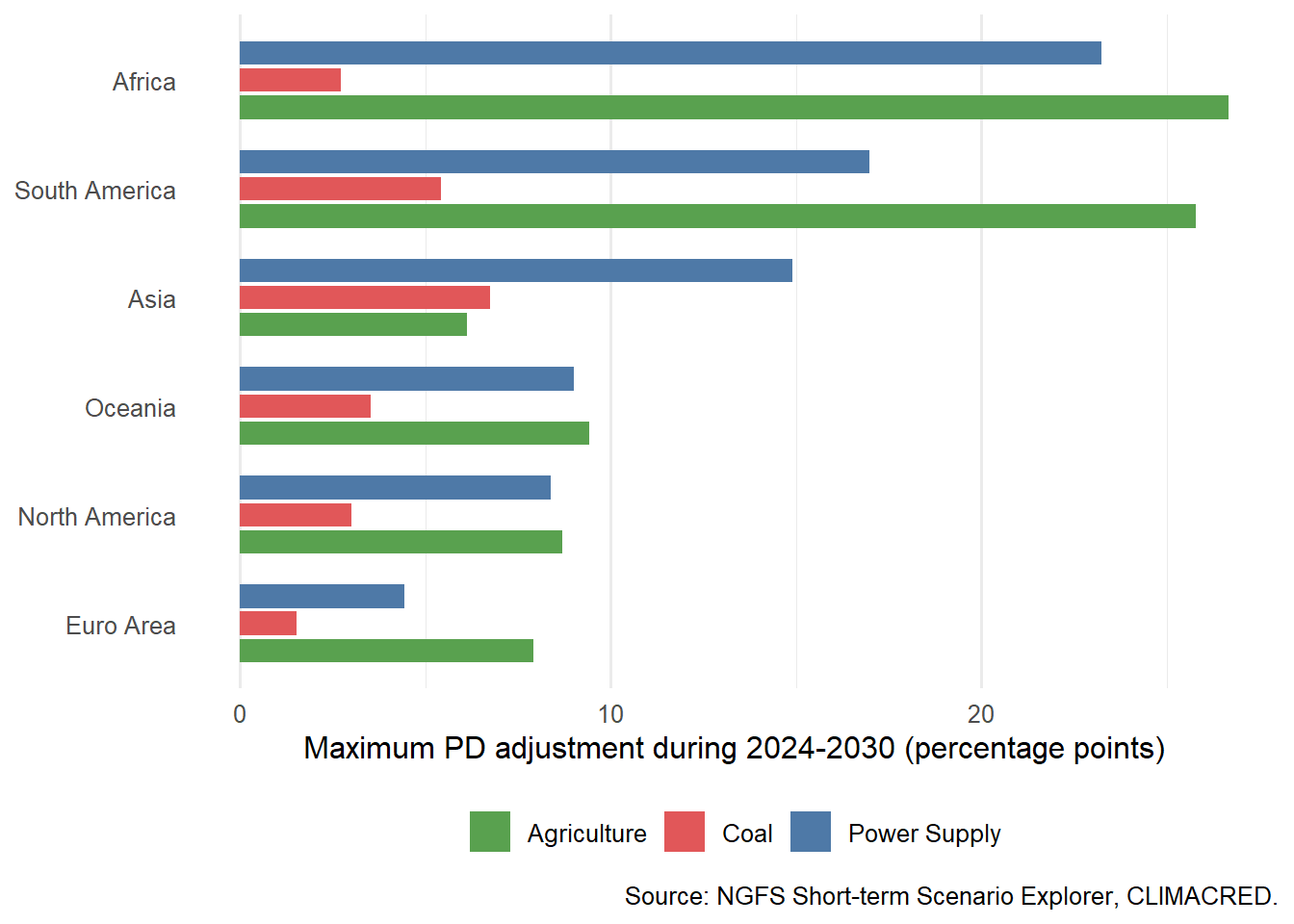
The global portfolio analysis uses World because the portfolio is global. Physical risk needs one extra check because physical events are regional. The DAPS runs in CLIMACRED are regional physical-stress runs. The download script saves a small DAPS sample, and the chapter compares the maximum PD adjustment over the short-term horizon.

Code

# These objects document the regional DAPS request saved by the download script.
daps_runs <- c(
  DAPS_AFR_R = 68,
  DAPS_ASIA = 69,
  DAPS_EUR = 70,
  DAPS_NAM = 71,
  DAPS_OCE = 72,
  DAPS_SAM = 73
)

daps_regions <- c(
  "Africa",
  "Asia",
  "Euro Area",
  "North America",
  "Oceania",
  "South America"
)

daps_region_map <- tibble::tibble(
  scenario = names(daps_runs),
  region = daps_regions
)

daps_variables <- as.vector(
  outer(
    "pd_adjustment",
    c("Agriculture", "Coal", "Power Supply"),
    paste,
    sep = "|"
  )
)

daps_raw <- utils::read.csv(
  file.path("data", "raw", "ngfs_climacred_daps_raw.csv"),
  stringsAsFactors = FALSE
)

daps_pd <- daps_raw |>
  tidyr::separate(
    variable,
    into = c("metric", "ngfs_sector"),
    sep = "\\|",
    remove = FALSE
  ) |>
  inner_join(daps_region_map, by = c("scenario", "region")) |>
  mutate(
    pd_adjustment = value / 100,
    region_label = case_when(
      scenario == "DAPS_AFR_R" ~ "Africa",
      scenario == "DAPS_ASIA" ~ "Asia",
      scenario == "DAPS_EUR" ~ "Euro Area",
      scenario == "DAPS_NAM" ~ "North America",
      scenario == "DAPS_OCE" ~ "Oceania",
      scenario == "DAPS_SAM" ~ "South America",
      TRUE ~ region
    )
  )

daps_summary <- daps_pd |>
  group_by(region_label, ngfs_sector) |>
  summarise(
    max_pd_adjustment = max(pd_adjustment, na.rm = TRUE),
    .groups = "drop"
  )

ggplot(
  daps_summary,
  aes(
    x = max_pd_adjustment * 100,
    y = reorder(region_label, max_pd_adjustment),
    fill = ngfs_sector
  )
) +
  geom_col(position = position_dodge(width = 0.75), width = 0.65) +
  scale_fill_manual(
    values = c(
      "Agriculture" = "#59A14F",
      "Coal" = "#E15759",
      "Power Supply" = "#4E79A7"
    )
  ) +
  labs(
    x = "Maximum PD adjustment during 2024-2030 (percentage points)",
    y = NULL,
    fill = NULL,
    caption = "Source: NGFS Short-term Scenario Explorer, CLIMACRED."
  ) +
  theme(
    legend.position = "bottom",
    legend.background = element_rect(fill = "white", colour = NA),
    panel.grid.major.y = element_blank()
  )

Figure 6.1: Regional physical-risk PD adjustments in selected CLIMACRED DAPS runs.

Figure Figure 6.1 serves as a diagnostic for the physical-risk channel. It also gives a useful modeling lesson. A transition scenario can often be represented at the global sector level. A physical scenario often needs location, because the same sector can face very different damage in different regions.

This has practical consequences because physical risk is tied to assets, operations, supply chains, and collateral. A global agriculture exposure is too broad for a loan officer who needs to understand drought, flood, or heat exposure. The DAPS diagnostic is therefore a warning about model granularity. Sector is usually enough to begin a transition-risk discussion. Physical risk often requires geography.

Code

physical_risk_data_requirements <- data.frame(
  Required_input = c(
    "Borrower geography",
    "Asset and collateral location",
    "Hazard intensity",
    "Vulnerability or damage function",
    "Insurance and recovery assumptions",
    "Business-interruption channel",
    "Credit translation",
    "Portfolio aggregation"
  ),
  `Why it matters for credit risk` = c(
    "The same sector can face different physical shocks in different regions.",
    "A borrower may be global, while the financed asset or collateral is local.",
    "Flood depth, heat stress, drought severity, or storm exposure determines the shock size.",
    "The hazard must be converted into damage, cost, lost revenue, or collateral impairment.",
    "Insurance and recovery affect LGD as well as borrower liquidity.",
    "Physical events can reduce revenue even when assets are not destroyed.",
    "The model needs a rule that maps physical damage into PD, LGD, spread, or rating migration.",
    "The final output must combine sector, geography, exposure, recovery, and dependence."
  ),
  check.names = FALSE
)

kable(
  physical_risk_data_requirements,
  caption = "Inputs needed to turn physical climate risk into a full credit-risk model.",
  row.names = FALSE
)

Inputs needed to turn physical climate risk into a full credit-risk model.
Required_input	Why it matters for credit risk
Borrower geography	The same sector can face different physical shocks in different regions.
Asset and collateral location	A borrower may be global, while the financed asset or collateral is local.
Hazard intensity	Flood depth, heat stress, drought severity, or storm exposure determines the shock size.
Vulnerability or damage function	The hazard must be converted into damage, cost, lost revenue, or collateral impairment.
Insurance and recovery assumptions	Insurance and recovery affect LGD as well as borrower liquidity.
Business-interruption channel	Physical events can reduce revenue even when assets are not destroyed.
Credit translation	The model needs a rule that maps physical damage into PD, LGD, spread, or rating migration.
Portfolio aggregation	The final output must combine sector, geography, exposure, recovery, and dependence.

This table explains why the chapter keeps the physical-risk block separate from the main expected-loss calculation. The teaching portfolio has sector exposures, but it does not contain borrower addresses, plant locations, collateral locations, or insurance information. Without those fields, forcing DAPS into the same portfolio expected-loss table would create precision that the data do not support.

If the bank had sector-region exposures, the workflow would extend naturally. Replace the global portfolio table with a sector-region portfolio, join the regional DAPS adjustments by sector and region, compute climate-adjusted PDs for each sector-region cell, and aggregate expected loss across the portfolio. The same expected-loss equation would apply. The richer data would determine where the physical shock enters.

6.4 Expected loss with climate-adjusted PDs

Expected loss starts with the same equation used throughout credit risk:

\[ EL_{i,t}=EAD_i \times LGD_i \times PD_{i,t}. \]

For a multi-year loan, a default in year $t$ can happen only if the borrower survived to the beginning of that year. Let $h_{i,t}$ denote the one-year conditional PD for sector $i$ in year $t$. The survival probability at the beginning of year $t$ is:

\[ S_{i,t-1} = \prod_{u=1}^{t-1}(1-h_{i,u}). \]

The marginal default probability in year $t$ is then:

\[ q_{i,t}=S_{i,t-1}h_{i,t}. \]

The present value of expected loss over a five-year horizon is:

\[ PV(EL_i) = \sum_{t=1}^{5} \frac{EAD_i \times LGD_i \times q_{i,t}}{(1+r)^t}. \]

This formula is worth reading slowly. The first year uses the first-year PD directly because $S_{i,0}=1$. Later years multiply the conditional PD by survival. That prevents us from counting a borrower as defaulting in year 4 after it already defaulted in year 2.

Code

pv_expected_loss <- function(pd_vector, ead, recovery, discount_rate) {
  h <- pmin(pmax(pd_vector, 0), 0.999)
  survival_start <- c(1, cumprod(1 - h)[-length(h)])
  marginal_pd <- survival_start * h
  discount <- 1 / (1 + discount_rate)^seq_along(h)

  sum(ead * (1 - recovery) * marginal_pd * discount)
}

risk_free_rate <- 0.04

horizon_loss <- climate_credit |>
  filter(year %in% horizon_years) |>
  arrange(scenario, portfolio_sector, year) |>
  group_by(
    scenario,
    scenario_label,
    portfolio_sector,
    ngfs_sector,
    ead,
    recovery
  ) |>
  summarise(
    pv_el_baseline = pv_expected_loss(
      baseline_pd,
      first(ead),
      first(recovery),
      risk_free_rate
    ),
    pv_el_climate = pv_expected_loss(
      climate_pd,
      first(ead),
      first(recovery),
      risk_free_rate
    ),
    incremental_pv_el = pv_el_climate - pv_el_baseline,
    .groups = "drop"
  )

portfolio_horizon_loss <- horizon_loss |>
  group_by(scenario_label) |>
  summarise(
    baseline_pv_el = sum(pv_el_baseline),
    climate_pv_el = sum(pv_el_climate),
    underestimated_pv_el = sum(incremental_pv_el),
    increase = climate_pv_el / baseline_pv_el - 1,
    .groups = "drop"
  )

largest_underestimate <- portfolio_horizon_loss |>
  arrange(desc(underestimated_pv_el)) |>
  slice(1)

top_sector_increase <- horizon_loss |>
  arrange(desc(incremental_pv_el)) |>
  slice(1)

coal_hwtp_path <- climate_credit |>
  filter(
    scenario == "HWTP",
    portfolio_sector == "Coal",
    year %in% horizon_years
  ) |>
  arrange(year)

coal_hwtp_survival_start <- c(
  1,
  cumprod(1 - coal_hwtp_path$climate_pd)[-length(coal_hwtp_path$climate_pd)]
)
coal_hwtp_marginal_pd <- coal_hwtp_survival_start * coal_hwtp_path$climate_pd
coal_hwtp_discount <- 1 / (1 + risk_free_rate)^seq_along(coal_hwtp_path$year)
coal_hwtp_lgd <- 1 - coal_hwtp_path$recovery
coal_hwtp_pv_el <- coal_hwtp_path$ead *
  coal_hwtp_lgd *
  coal_hwtp_marginal_pd *
  coal_hwtp_discount

coal_hwtp_el_steps <- data.frame(
  Year = coal_hwtp_path$year,
  `Climate PD` = fmt_pct(coal_hwtp_path$climate_pd, 2),
  `Survival at start` = fmt_pct(coal_hwtp_survival_start, 2),
  `Marginal PD` = fmt_pct(coal_hwtp_marginal_pd, 2),
  EAD = fmt_usd_m(coal_hwtp_path$ead),
  LGD = fmt_pct(coal_hwtp_lgd, 1),
  `Discount factor` = fmt_num(coal_hwtp_discount, 4),
  `PV expected loss` = fmt_usd_m(coal_hwtp_pv_el)
)

portfolio_horizon_loss |>
  transmute(
    Scenario = scenario_label,
    `PV expected loss without climate` = fmt_usd_m(baseline_pv_el),
    `PV expected loss with climate` = fmt_usd_m(climate_pv_el),
    `Underestimated PV expected loss` = fmt_usd_m(underestimated_pv_el),
    `Relative increase` = fmt_pct(increase, 1)
  ) |>
  kable(
    caption = "Five-year portfolio expected loss with and without the CLIMACRED climate adjustment."
  )

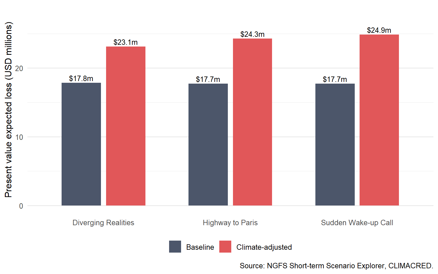
Five-year portfolio expected loss with and without the CLIMACRED climate adjustment.
Scenario	PV expected loss without climate	PV expected loss with climate	Underestimated PV expected loss	Relative increase
Diverging Realities	$17.85m	$23.11m	$5.26m	29.5%
Highway to Paris	$17.71m	$24.30m	$6.59m	37.2%
Sudden Wake-up Call	$17.72m	$24.87m	$7.15m	40.3%

Code

kable(
  coal_hwtp_el_steps,
  caption = "Coal expected-loss mechanics under Highway to Paris.",
  row.names = FALSE
)

Coal expected-loss mechanics under Highway to Paris.
Year	Climate.PD	Survival.at.start	Marginal.PD	EAD	LGD	Discount.factor	PV.expected.loss
2026	32.58%	100.00%	32.58%	$10.00m	65.0%	0.9615	$2.04m
2027	39.92%	67.42%	26.91%	$10.00m	65.0%	0.9246	$1.62m
2028	39.76%	40.51%	16.10%	$10.00m	65.0%	0.8890	$0.93m
2029	42.02%	24.40%	10.25%	$10.00m	65.0%	0.8548	$0.57m
2030	42.23%	14.15%	5.97%	$10.00m	65.0%	0.8219	$0.32m

The calculation answers the first question of the chapter. Ignoring climate risk means using the baseline PD path and missing the additional expected loss generated by the scenario PD adjustment. The amount missed becomes a dollar present value on the same portfolio used by the bank.

In this portfolio, the largest underestimation occurs under the Sudden Wake-up Call scenario. The five-year present value of expected loss rises by $7.15m, which is a 40.3% increase relative to the baseline calculation. That is the kind of number that can enter a credit memo, a portfolio review, or a stress-testing dashboard. It is also why climate credit risk should be expressed in ordinary credit units. A committee can debate a dollar expected-loss increase much more clearly than an abstract climate score.

The Coal table shows the same calculation inside one sector. The climate PD is treated as a one-year conditional PD. The survival column prevents double counting across years, the marginal PD gives the probability weight for the default year, and the last column converts that probability into discounted expected loss using EAD, LGD, and the discount factor.

Code

portfolio_horizon_loss |>
  tidyr::pivot_longer(
    cols = c(baseline_pv_el, climate_pv_el),
    names_to = "case",
    values_to = "pv_expected_loss"
  ) |>
  mutate(
    case = recode(
      case,
      baseline_pv_el = "Baseline",
      climate_pv_el = "Climate-adjusted"
    )
  ) |>
  ggplot(
    aes(
      x = scenario_label,
      y = pv_expected_loss / 1e6,
      fill = case
    )
  ) +
  geom_col(
    position = position_dodge(width = 0.7),
    width = 0.62
  ) +
  geom_text(
    aes(label = paste0("$", fmt_num(pv_expected_loss / 1e6, 1), "m")),
    position = position_dodge(width = 0.7),
    vjust = -0.35,
    size = 3.4
  ) +
  scale_fill_manual(
    values = c(
      "Baseline" = "#4C566A",
      "Climate-adjusted" = "#E15759"
    )
  ) +
  labs(
    x = NULL,
    y = "Present value expected loss (USD millions)",
    fill = NULL,
    caption = "Source: NGFS Short-term Scenario Explorer, CLIMACRED."
  ) +
  expand_limits(y = max(portfolio_horizon_loss$climate_pv_el) / 1e6 * 1.12) +
  theme(
    legend.position = "bottom",
    legend.background = element_rect(fill = "white", colour = NA),
    panel.grid.major.x = element_blank()
  )

Figure 6.2: Portfolio expected loss with and without CLIMACRED climate adjustments.

Figure Figure 6.2 keeps exposures and recoveries fixed. The difference between the baseline bars and climate-adjusted bars comes only from the climate PD adjustment. That is why the chart is useful for a risk committee: it isolates the credit effect of the scenario. The climate overlay is material in this teaching portfolio. It changes the scale of expected loss enough to affect pricing, limits, provisions, or hedging discussions.

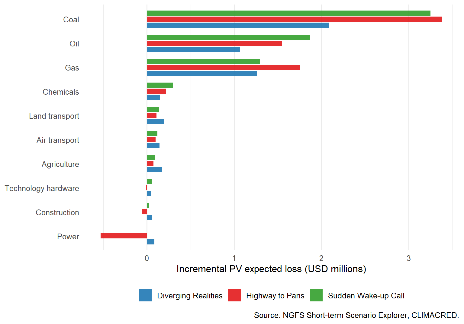
6.5 Which sectors drive the increase

The portfolio total answers how much risk increases. A risk manager also needs to know where the increase comes from. The sector-level expected loss decomposition is:

\[ \Delta PV(EL_i) = PV(EL_i^{climate})-PV(EL_i^{base}). \]

This is a contribution measure. A sector can contribute more because its climate PD adjustment is high, because its exposure is large, because its recovery is low, or because all three happen at the same time.

Code

horizon_loss |>
  ggplot(
    aes(
      x = incremental_pv_el / 1e6,
      y = reorder(portfolio_sector, incremental_pv_el),
      fill = scenario_label
    )
  ) +
  geom_col(
    position = position_dodge(width = 0.75),
    width = 0.65,
    alpha = 0.9
  ) +
  scale_fill_manual(values = book_palette[names(book_palette) != "Baseline"]) +
  labs(
    x = "Incremental PV expected loss (USD millions)",
    y = NULL,
    fill = NULL,
    caption = "Source: NGFS Short-term Scenario Explorer, CLIMACRED."
  ) +
  theme(
    legend.position = "bottom",
    legend.background = element_rect(fill = "white", colour = NA),
    panel.grid.major.y = element_blank()
  )

Figure 6.3: Sector contributions to incremental climate expected loss.

The ranking in Figure Figure 6.3 is the actionable part. A portfolio manager can go beyond saying that the climate scenario is adverse. The chart says which sectors explain the underestimation. That can lead to exposure limits, extra monitoring, sector overlays, loan pricing changes, collateral review, or CDS hedging.

Negative bars are possible. They mean that the scenario reduces the model-implied PD for that sector relative to BAU. In a transition scenario, a cleaner or transition-benefiting sector can improve while fossil sectors deteriorate. The portfolio result is the net effect across sectors.

For the full set of scenarios in this chapter, the largest single positive contribution comes from Coal under Highway to Paris, with an incremental present value expected loss of $3.38m. That statement turns a broad climate-risk concern into a specific sector and scenario combination that drives the result.

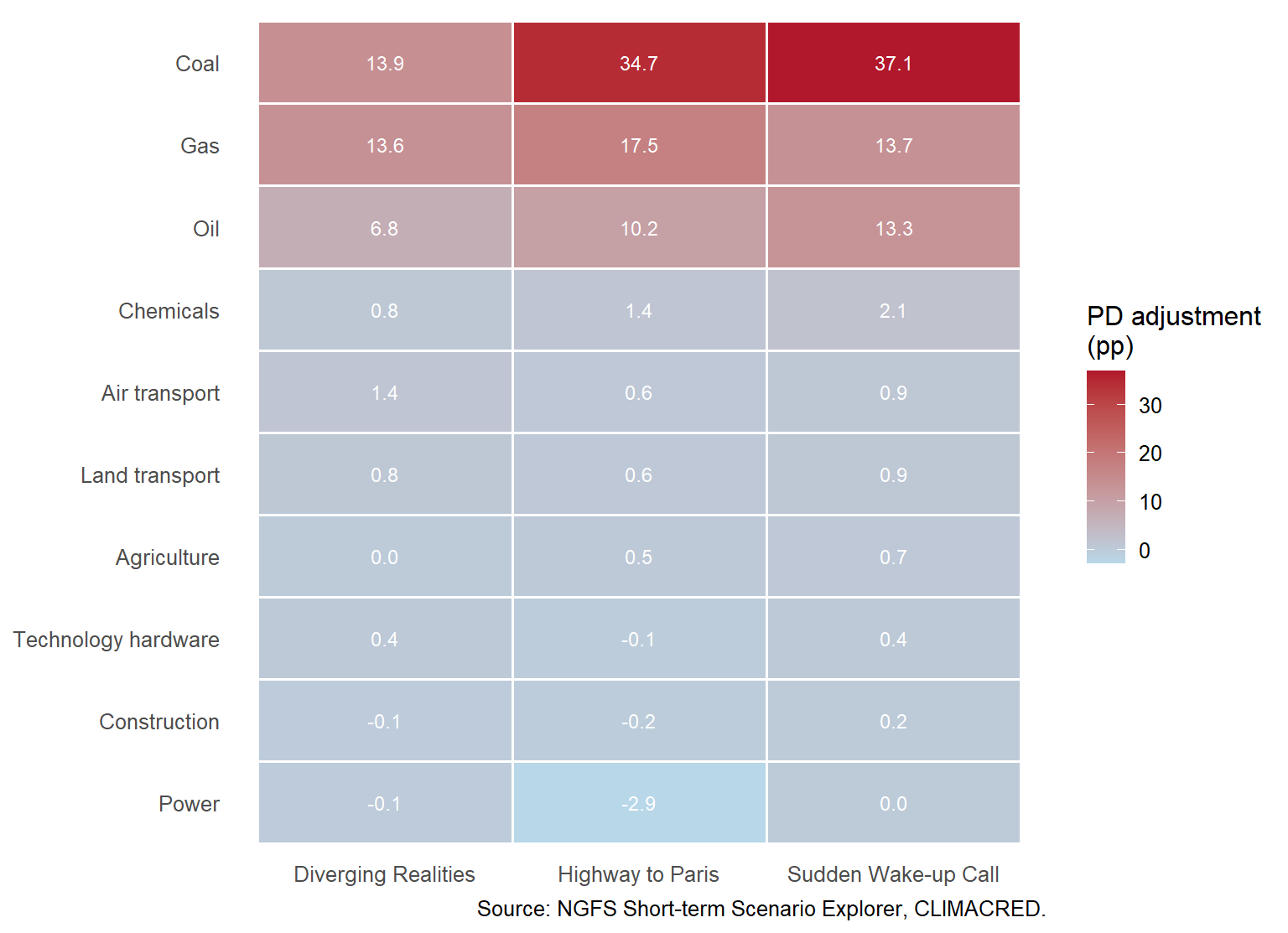
The next figure separates the PD adjustment itself from exposure size. It shows the 2030 climate PD adjustment by scenario and sector. A dark cell means that the climate scenario adds a large number of percentage points to the baseline PD.

Code

pd_heatmap <- climate_credit |>
  filter(year == 2030) |>
  mutate(
    pd_adjustment_pp = 100 * pd_adjustment
  )

ggplot(
  pd_heatmap,
  aes(
    x = scenario_label,
    y = reorder(portfolio_sector, pd_adjustment_pp),
    fill = pd_adjustment_pp
  )
) +
  geom_tile(color = "white", linewidth = 0.6) +
  geom_text(
    aes(label = fmt_num(pd_adjustment_pp, 1)),
    size = 3.2,
    color = "white"
  ) +
  scale_fill_gradient(
    low = "#B8D7E8",
    high = "#B2182B",
    name = "PD adjustment\n(pp)"
  ) +
  labs(
    x = NULL,
    y = NULL,
    caption = "Source: NGFS Short-term Scenario Explorer, CLIMACRED."
  ) +
  theme(
    legend.position = "right",
    legend.background = element_rect(fill = "white", colour = NA),
    panel.grid = element_blank()
  )

Figure 6.4: Climate PD adjustments by scenario and sector in 2030.

Figure Figure 6.4 helps distinguish two ideas. A sector can be climate-sensitive because its PD adjustment is large. It can still be a smaller portfolio contributor if the exposure is small or the recovery is high. Expected loss combines both the scenario shock and the portfolio weights.

That distinction is important for governance. A supervisor or senior risk manager may ask for both views. The heatmap answers where the scenario shock is most severe. The contribution chart answers where the portfolio loses the most money. A sector with a large PD shock but a small exposure can be a warning signal without being the largest current loss contributor. A sector with moderate PD stress and large exposure can dominate the portfolio result.

Code

path_sectors <- c(
  "Coal",
  "Power Supply",
  "Land transport",
  "Computer, electronic and optical products"
)

pd_path <- climate_credit |>
  filter(
    scenario == "HWTP",
    ngfs_sector %in% path_sectors
  ) |>
  select(
    year,
    portfolio_sector,
    baseline_pd,
    climate_pd
  ) |>
  tidyr::pivot_longer(
    cols = c(baseline_pd, climate_pd),
    names_to = "case",
    values_to = "pd"
  ) |>
  mutate(
    case = recode(
      case,
      baseline_pd = "Baseline",
      climate_pd = "Climate-adjusted"
    )
  )

ggplot(
  pd_path,
  aes(
    x = year,
    y = pd,
    color = case,
    linetype = case
  )
) +
  geom_line(linewidth = 0.9) +
  geom_point(size = 2.2, alpha = 0.85) +
  facet_wrap(~ portfolio_sector, ncol = 2) +
  scale_y_continuous(labels = percent_format(accuracy = 1)) +
  scale_color_manual(
    values = c(
      "Baseline" = "#4C566A",
      "Climate-adjusted" = "#E15759"
    ),
    breaks = c("Baseline", "Climate-adjusted")
  ) +
  scale_linetype_manual(
    values = c(
      "Baseline" = "dashed",
      "Climate-adjusted" = "solid"
    ),
    breaks = c("Baseline", "Climate-adjusted")
  ) +
  labs(
    x = NULL,
    y = "One-year PD",
    color = NULL,
    linetype = NULL,
    caption = "Source: NGFS Short-term Scenario Explorer, CLIMACRED. Scenario: Highway to Paris."
  ) +
  theme(
    legend.position = "bottom",
    legend.background = element_rect(fill = "white", colour = NA),
    panel.grid.minor = element_blank()
  )

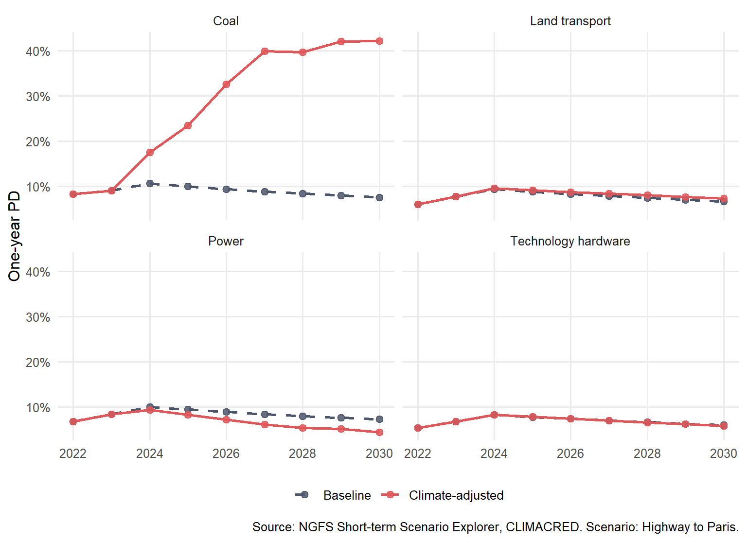
Figure 6.5: Baseline and climate-adjusted PD paths under Highway to Paris.

Figure Figure 6.5 shows that the timing of the adjustment also changes the credit interpretation. Coal is repriced much more severely than technology hardware in this scenario, and the gap opens over the short-term horizon. That time path affects credit decisions. A one-year loan, a five-year bond, and a long-dated project-finance exposure face different amounts of climate-adjusted credit risk. Maturity is therefore part of the interpretation.

6.6 Spreads, bond prices, and CDS compensation

Chapter 4 showed that a default probability becomes a spread only after we specify recovery, discounting, and the promised cash flows. CLIMACRED gives a market-style output directly through corporate_bond_spread_adjustment and corporate_bond_price_rel_adjustment. We can use those variables as a market translation of the PD shock.

The spread adjustment is measured in percentage points. A value of 1.25 means 125 basis points. The bond price adjustment is measured as a percent change relative to BAU. A value of -5 means the bond price is 5% lower than in the baseline.

Code

market_snapshot <- climate_credit |>
  filter(year == 2030) |>
  transmute(
    scenario_label,
    portfolio_sector,
    spread_adjustment_bps = corporate_bond_spread_adjustment * 10000,
    price_adjustment_pct = corporate_bond_price_rel_adjustment * 100
  )

top_market_move <- market_snapshot |>
  arrange(desc(spread_adjustment_bps)) |>
  slice(1)

market_snapshot |>
  arrange(scenario_label, desc(spread_adjustment_bps)) |>
  group_by(scenario_label) |>
  slice_head(n = 3) |>
  ungroup() |>
  transmute(
    Scenario = scenario_label,
    Sector = portfolio_sector,
    `Spread adjustment` = fmt_bps_label(spread_adjustment_bps, 0),
    `Bond price adjustment` = fmt_pct(price_adjustment_pct / 100, 2)
  ) |>
  kable(
    caption = "Largest 2030 CLIMACRED corporate bond spread adjustments by scenario."
  )

Largest 2030 CLIMACRED corporate bond spread adjustments by scenario.
Scenario	Sector	Spread adjustment	Bond price adjustment
Diverging Realities	Gas	826 bps	-8.07%
Diverging Realities	Coal	596 bps	-8.39%
Diverging Realities	Oil	347 bps	-3.94%
Highway to Paris	Coal	1818 bps	-19.75%
Highway to Paris	Gas	1014 bps	-9.81%
Highway to Paris	Oil	572 bps	-5.76%
Sudden Wake-up Call	Coal	1912 bps	-21.14%
Sudden Wake-up Call	Gas	807 bps	-7.60%
Sudden Wake-up Call	Oil	743 bps	-7.46%

The table moves from loan-style credit risk to market-style credit risk. Higher spread adjustments mean that investors require more compensation to hold the sector’s debt under the scenario. Negative bond price adjustments are the price counterpart of that repricing. In the chapter’s data, the largest 2030 spread adjustment is 1912 bps for Coal under Sudden Wake-up Call, with a bond price adjustment of -21.14%. That is economically large. It says that the climate scenario can affect both the banking book and the mark-to-market value of credit instruments.

Now connect the spread result to a CDS-style calculation. In a simple one-period approximation, a fair CDS spread is close to:

\[ s_{i,t}\approx LGD_i \times PD_{i,t}. \]

This approximation gives a bridge to the full CDS valuation logic developed in Chapter 4. It leaves out quarterly premium accrual and uses the same intuition behind a simple CDS spread. If climate risk raises PD, the protection premium that compensates the seller should also rise. The implied incremental CDS spread is:

\[ \Delta s_{i,t} \approx LGD_i \left( PD^{climate}_{i,t,s}-PD^{base}_{i,t,s} \right). \]

Code

spread_bridge <- climate_credit |>
  filter(year == 2030) |>
  mutate(
    cds_increment_bps = lgd * (climate_pd - baseline_pd) * 10000,
    ngfs_spread_bps = corporate_bond_spread_adjustment * 10000
  )

spread_bridge_gap <- spread_bridge |>
  mutate(spread_gap_bps = ngfs_spread_bps - cds_increment_bps)

largest_market_premium_gap <- spread_bridge_gap |>
  arrange(desc(spread_gap_bps)) |>
  slice(1)

largest_default_loss_gap <- spread_bridge_gap |>
  arrange(spread_gap_bps) |>
  slice(1)

ggplot(
  spread_bridge,
  aes(
    x = cds_increment_bps,
    y = ngfs_spread_bps,
    color = scenario_label
  )
) +
  geom_abline(
    slope = 1,
    intercept = 0,
    linetype = "dashed",
    color = "#666666",
    linewidth = 0.7
  ) +
  geom_point(size = 3, alpha = 0.85) +
  facet_wrap(~ scenario_label) +
  scale_color_manual(values = book_palette[names(book_palette) != "Baseline"]) +
  labs(
    x = "Incremental CDS-style spread from PD x LGD (bps)",
    y = "NGFS corporate bond spread adjustment (bps)",
    color = NULL,
    caption = "Source: NGFS Short-term Scenario Explorer, CLIMACRED."
  ) +
  theme(
    legend.position = "none",
    legend.background = element_rect(fill = "white", colour = NA),
    panel.grid.minor = element_blank()
  )

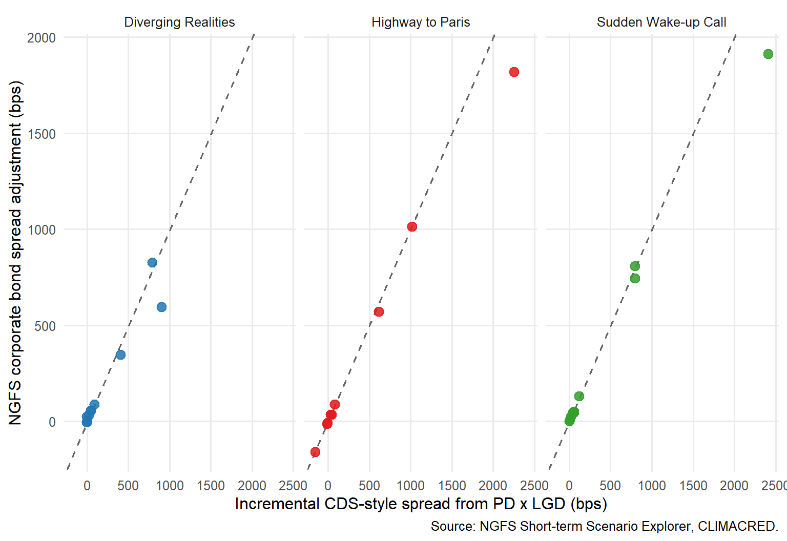
Figure 6.6: CLIMACRED bond spread adjustments compared with a CDS-style PD x LGD benchmark.

The dashed line in Figure Figure 6.6 is a reference line. The x-axis is the simple CDS-style PD-times-LGD calculation from this chapter. The y-axis is the CLIMACRED corporate bond spread adjustment. If the two are close, the spread move is largely aligned with expected default loss. If the NGFS spread adjustment is higher, the market-style output is also capturing discount-rate, mark-to-market, maturity, policy, or risk-premium effects. If it is lower, the bond adjustment is smaller than the simple PD-times-LGD benchmark.

The largest positive gap in this comparison is 35 bps for Gas under Diverging Realities. In that case, the NGFS market-style spread adjustment is above the simple default-loss benchmark. The largest negative gap is -496 bps for Coal under Sudden Wake-up Call, where the simple PD-times-LGD benchmark is larger than the NGFS spread adjustment. These gaps are diagnostics, not trading signals. They tell the analyst where the market-style scenario output and the default-loss approximation tell different stories.

This comparison is useful because it shows how a climate PD shock can travel into different credit instruments. A bank loan uses PD, LGD, and EAD. A corporate bond uses spread and price. A CDS uses protection payments and premium legs. The same climate scenario can be read through all three lenses.

For a practitioner, this bridge creates a practical diagnostic. If the model-implied PD shock suggests a much larger CDS-style spread than the observed or scenario-implied bond spread, the bond may be undercompensating investors for default loss. If the market-style spread is much larger, investors may be pricing additional risks beyond default loss, such as liquidity, uncertainty about transition policy, or broader risk premia. The purpose is to make the climate credit channel visible in the units used by credit markets before moving to full bond or CDS valuation.

6.7 Portfolio loss simulation

Expected loss is the average. Risk management also needs the distribution. A portfolio can have the same expected loss and still have very different tail risk if defaults cluster. To keep the simulation aligned with the copula chapter, we use a one-factor Gaussian default model:

\[ X_i=\sqrt{\rho}Z+\sqrt{1-\rho}\epsilon_i. \]

The common factor $Z$ represents the shared credit environment. The idiosyncratic shock $\epsilon_i$ is sector-specific. Sector $i$ defaults in the simulation if:

\[ X_i < \Phi^{-1}(PD_i). \]

The threshold is lower for safer sectors and higher for riskier sectors. Raising $PD_i$ through the climate adjustment makes default more likely in the simulation.

Code

simulate_climate_losses <- function(pd_baseline,
                                    pd_climate,
                                    ead,
                                    recovery,
                                    rho = 0.25,
                                    n_sims = 50000,
                                    seed = 202606) {
  set.seed(seed)

  n_sectors <- length(pd_baseline)
  common_factor <- rnorm(n_sims)
  idiosyncratic <- matrix(
    rnorm(n_sims * n_sectors),
    nrow = n_sims,
    ncol = n_sectors
  )

  credit_score <- sqrt(rho) * common_factor +
    sqrt(1 - rho) * idiosyncratic

  loss_given_default <- ead * (1 - recovery)

  baseline_defaults <- sweep(
    credit_score,
    2,
    qnorm(pd_baseline),
    "<"
  )

  climate_defaults <- sweep(
    credit_score,
    2,
    qnorm(pd_climate),
    "<"
  )

  tibble::tibble(
    case = rep(c("Baseline", "Climate-adjusted"), each = n_sims),
    loss = c(
      as.numeric(baseline_defaults %*% loss_given_default),
      as.numeric(climate_defaults %*% loss_given_default)
    )
  )
}

simulation_input <- climate_credit |>
  filter(
    year == 2030,
    scenario == "HWTP"
  ) |>
  arrange(portfolio_sector)

simulated_losses <- simulate_climate_losses(
  pd_baseline = simulation_input$baseline_pd,
  pd_climate = simulation_input$climate_pd,
  ead = simulation_input$ead,
  recovery = simulation_input$recovery
)

loss_summary <- simulated_losses |>
  group_by(case) |>
  summarise(
    mean_loss = mean(loss),
    var_95 = as.numeric(quantile(loss, 0.95)),
    es_95 = mean(loss[loss >= as.numeric(quantile(loss, 0.95))]),
    .groups = "drop"
  )

loss_lift <- loss_summary |>
  mutate(case_id = if_else(case == "Baseline", "baseline", "climate")) |>
  select(case_id, mean_loss, var_95, es_95) |>
  tidyr::pivot_wider(
    names_from = case_id,
    values_from = c(mean_loss, var_95, es_95)
  ) |>
  mutate(
    mean_increase = mean_loss_climate - mean_loss_baseline,
    var_increase = var_95_climate - var_95_baseline,
    es_increase = es_95_climate - es_95_baseline
  )

loss_summary |>
  transmute(
    Case = case,
    `Mean loss` = fmt_usd_m(mean_loss),
    `95% VaR` = fmt_usd_m(var_95),
    `95% expected shortfall` = fmt_usd_m(es_95)
  ) |>
  kable(
    caption = "One-year simulated portfolio loss in 2030 under Highway to Paris."
  )

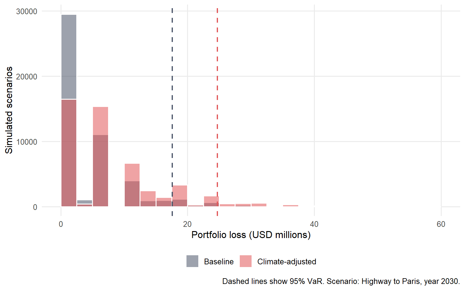
One-year simulated portfolio loss in 2030 under Highway to Paris.
Case	Mean loss	95% VaR	95% expected shortfall
Baseline	$4.10m	$17.60m	$23.16m
Climate-adjusted	$8.12m	$24.70m	$30.03m

The simulation uses the same random credit states for the baseline and climate-adjusted cases. That design is deliberate. It lets the comparison focus on the PD change and removes random simulation noise from the comparison.

The result changes both the average and the tail. Mean one-year loss increases by $4.02m. The 95% VaR increases by $7.10m, and the 95% expected shortfall increases by $6.86m. That is a different message from the expected-loss table. Expected loss is useful for pricing and provisioning. VaR and expected shortfall are useful for risk appetite, capital planning, and stress testing.

Code

ggplot(
  simulated_losses,
  aes(
    x = loss / 1e6,
    fill = case
  )
) +
  geom_histogram(
    binwidth = 2.5,
    position = "identity",
    alpha = 0.55,
    boundary = 0,
    color = "white"
  ) +
  geom_vline(
    data = loss_summary,
    aes(xintercept = var_95 / 1e6, color = case),
    linetype = "dashed",
    linewidth = 0.8
  ) +
  scale_fill_manual(
    values = c(
      "Baseline" = "#4C566A",
      "Climate-adjusted" = "#E15759"
    ),
    breaks = c("Baseline", "Climate-adjusted")
  ) +
  scale_color_manual(
    values = c(
      "Baseline" = "#4C566A",
      "Climate-adjusted" = "#E15759"
    ),
    breaks = c("Baseline", "Climate-adjusted")
  ) +
  labs(
    x = "Portfolio loss (USD millions)",
    y = "Simulated scenarios",
    fill = NULL,
    color = NULL,
    caption = "Dashed lines show 95% VaR. Scenario: Highway to Paris, year 2030."
  ) +
  guides(color = "none") +
  theme(
    legend.position = "bottom",
    legend.background = element_rect(fill = "white", colour = NA),
    panel.grid.minor = element_blank()
  )

Figure 6.7: Baseline and climate-adjusted portfolio loss distributions under Highway to Paris.

Figure Figure 6.7 turns the expected-loss result into a risk-distribution result. Climate-adjusted PDs move probability mass toward larger losses. The VaR line also moves because more scenarios contain multiple sector defaults. This is the portfolio version of the same story: climate risk changes credit analysis when it changes the probability, timing, clustering, or severity of credit losses.

The plot also shows why a climate overlay should be connected to portfolio models as well as individual borrower PDs. A small loan-level PD change may look manageable in isolation. In a concentrated portfolio with correlated defaults, many small changes can move the tail. That is the link between this chapter and the copula chapter.

6.8 What the chapter adds

The chapter adds a climate layer to the credit-risk toolkit built earlier in the book. Chapter 1 and Chapter 2 estimate borrower default risk from data. Chapter 3 connects corporate default to firm value and volatility. Chapter 4 translates default risk into bond spreads and CDS valuation. Chapter 5 turns individual PDs into portfolio loss distributions. This chapter uses public climate-scenario data to shock PDs, expected loss, spreads, bond prices, and simulated portfolio losses.

The key modeling discipline is simple:

Start from a credit quantity that has financial meaning.
Use a public climate scenario to change that credit quantity.
Convert the change into dollars, spreads, prices, or loss distributions.
Decompose the result by sector or geography so the output can guide action.

The most important limitation is interpretation. The NGFS scenario serves as a stress-testing input, separate from a trading signal. The portfolio is a teaching portfolio. The recoveries are analyst assumptions. The Gaussian simulation is deliberately simple. The physical-risk block is diagnostic because the teaching portfolio has no borrower or collateral geography. A production model would need borrower-level exposures, maturities, collateral, geographic locations, sector taxonomies, rating migration, balance-sheet dynamics, current market prices, scenario governance, and model validation.

Those limitations clarify the purpose of the chapter. The objective is to show how climate data can enter a credit-risk workflow in a way that is transparent, reproducible, and financially interpretable.