5 The Gaussian copula model for portfolio credit risk

The previous chapters focused on one borrower at a time. A logistic model estimates an individual default probability from borrower characteristics. A tree-based model does the same with a more flexible prediction function. The Merton model links a firm’s equity, assets, debt, volatility, and default probability. The credit-spread chapter then shows how market prices, bond spreads, and CDS spreads can translate default risk into compensation. A lender, bank, or investor usually holds a portfolio, so portfolio credit risk asks a different question.

Given individual default probabilities, exposures, recoveries, and a rule for how borrowers can default together, what is the distribution of portfolio defaults and credit losses?

This chapter studies the Gaussian copula as a way to answer that portfolio question. The model starts with individual cumulative PDs and then builds scenarios in which several borrowers can default together. A scenario is one possible credit environment for the portfolio. In each scenario, every firm receives a standardized credit-state score. Low scores represent weak credit conditions, and a firm defaults when its score falls below the threshold implied by its own PD.

The model is useful because the simulated scenarios have to pass two checks. First, each firm should default with the cumulative PD that we put into the model. Second, changing the correlation input should change co-default behavior while leaving the individual PDs unchanged. The chapter checks both points numerically before using the model for portfolio losses. The final sections use a t-copula extension to show how joint tail behavior changes capital.

The starting point is Hull’s discussion of default correlation in section 24.8 of (Hull 2022). Defaults tend to cluster because firms can share industries, countries, funding conditions, macroeconomic shocks, or direct business links. The Gaussian copula gives us a way to turn that financial idea into code.

The early references give the origin of the model. CreditMetrics, developed by J.P. Morgan, framed credit risk as a portfolio VaR problem with credit-event correlations, scenario generation, credit limits, and economic capital (Gupton et al. 1997). Li’s copula approach connected marginal default information with a joint default distribution for products such as credit default swaps and first-to-default contracts (Li 2000). The Basel II explanatory note gives the economic logic behind a related one-factor credit portfolio model, where a PD is transformed into a default threshold and a common risk factor represents adverse economic conditions (Basel Committee on Banking Supervision 2005).

The reason to keep the model in a current credit-risk chapter is practical. Current risk software still implements copula-based credit simulations. MathWorks documents a creditDefaultCopula workflow for simulating default losses, portfolio risk measures, confidence bands, and risk contributions (MathWorks 2026). CCruncher is an open-source credit portfolio engine, updated in 2025, that simulates portfolio loss distributions with Gaussian and t copulas, PDs, EADs, LGDs, ratings, sector correlations, VaR, and Expected Shortfall (CCruncher 2025). Current Basel Framework IRB risk-weight functions also keep PD, LGD, EAD, maturity, and asset-correlation inputs close to regulatory practice (Basel Committee on Banking Supervision 2026). Recent research uses factor copulas and CDS spreads to model joint and conditional distress probabilities for European and U.S. banks, including stress episodes such as COVID-19, the 2022 rate-hike period, and the 2023 banking crisis (Nguyen et al. 2024). This chapter uses that same portfolio question in a simpler teaching setting.

The route through the chapter is sequential. First, we define the portfolio co-default problem and separate marginal default risk, dependence, exposure, recovery, and loss. Second, we rebuild Hull’s Example 24.7 by converting cumulative PDs into normal default thresholds. Third, we check the threshold rule for one firm and then show with two firms how shared credit shocks change joint defaults while preserving individual PDs. Fourth, we extend the simulation to ten firms and translate default counts into portfolio losses. Fifth, we change exposure weights to isolate concentration risk. Sixth, we compare Gaussian and t-copulas to show how joint tail behavior changes loss estimates. Finally, we connect the simulation logic to Credit VaR, expected shortfall, and economic capital.

5.1 Default correlation and the portfolio problem

Imagine a bank with loans to ten manufacturing firms. The credit team may know the 5-year cumulative PD of each firm. That information is useful, but it answers a borrower-level question. It says how often each name defaults over five years. The portfolio manager also needs a portfolio-level answer. Do defaults tend to arrive one by one, or can several borrowers fail in the same bad credit environment?

That second question is the co-default problem. Co-default means that several borrowers default within the same horizon. A lender can absorb isolated defaults more easily than a cluster of defaults arriving together, so co-default directly affects portfolio loss risk.

Defaults cluster for economic reasons. Firms in the same industry can face the same fall in demand. Firms in the same country can face the same interest-rate, exchange-rate, or funding shock. A supplier can be hurt when a large customer defaults. A borrower that depends on refinancing can become fragile when market liquidity dries up. These shared forces leave diversification incomplete even when a portfolio contains many borrowers.

The Gaussian copula turns this idea into a disciplined scenario model. In each scenario, firm $i$ receives a credit-state score, denoted $X_i$. Think of $X_i$ as a compact summary of the credit environment facing that firm in that scenario. It stands in for the combined effect of demand, margins, funding access, refinancing conditions, collateral values, sector stress, and other credit-relevant forces. A high value of $X_i$ means a strong credit state. A low value means a weak credit state.

The modeling target is deliberately narrow: one standardized credit-state score per firm and per scenario. The default threshold then gives that score financial meaning. If a firm’s 5-year cumulative PD is 15%, the threshold is chosen so that the worst 15% of simulated credit states are counted as defaults by year 5.

Simulation is useful here because a portfolio has many possible default combinations. With ten firms there are already $2^{10}=1{,}024$ possible default sets by a given horizon. The simulation creates many credit scenarios, applies the same default rule in each scenario, and counts the resulting portfolio defaults. The first check is mechanical: simulated default frequencies should reproduce the input PDs. After that check passes, the financial question is which value of $\rho$ is a reasonable description of common credit stress.

Dependence has a concrete credit-risk meaning here. The firms’ credit-state scores tend to be weak together more often, or less often, than they would under independence. The copula correlation $\rho$ controls that shared movement. If $\rho$ is high, a bad scenario for one borrower is more likely to be a bad scenario for other borrowers too. The Gaussian copula procedure starts from individual cumulative PDs, converts them into default thresholds, draws correlated credit-state scores, and records which firms default in each scenario. Once we know which firms default, exposures and recoveries convert those default events into portfolio losses.

For the equal-correlation examples in this chapter, a simple one-factor version makes the shared shock visible:

\[ X_i=\sqrt{\rho}\,Z_0+\sqrt{1-\rho}\,Z_i. \]

The score $X_i$ is the simulated credit state of firm $i$. The variable $Z_0$ is the common credit shock in the scenario, such as a recession, a funding squeeze, or a sector-wide stress event. The variable $Z_i$ is the firm-specific shock. If $Z_0$ is very low, many firms receive weak credit-state scores in the same simulation. The parameter $\rho$ controls how much each firm’s score depends on that common shock. This is the mechanism that creates co-default risk.

The main simulation functions are shown below. They are reused throughout the chapter. The first function creates an equal-correlation matrix. The second function draws correlated credit-state scores. The third function converts those scores into default indicators by comparing each score with its default threshold. The remaining functions summarize default counts, convert defaults into portfolio losses, and report tail-risk measures.

Code

make_correlation_matrix <- function(n_firms, rho) {
  sigma <- matrix(rho, nrow = n_firms, ncol = n_firms)
  diag(sigma) <- 1
  sigma
}

simulate_latent_credit <- function(n_sims, n_firms, rho, seed = 130575) {
  set.seed(seed)
  MASS::mvrnorm(
    n = n_sims,
    mu = rep(0, n_firms),
    Sigma = make_correlation_matrix(n_firms, rho)
  )
}

make_default_matrix <- function(latent_credit, threshold) {
  latent_credit <= threshold
}

summarize_default_counts <- function(default_matrix) {
  default_count <- rowSums(default_matrix)
  count_table <- as.data.frame(table(default_count))
  names(count_table) <- c("defaults", "frequency")
  count_table$defaults <- as.integer(as.character(count_table$defaults))
  count_table$probability <- count_table$frequency / nrow(default_matrix)
  count_table
}

portfolio_losses <- function(default_matrix, ead, recovery) {
  lgd_amount <- ead * (1 - recovery)
  as.numeric(default_matrix %*% lgd_amount)
}

loss_risk_summary <- function(losses) {
  var_95 <- unname(quantile(losses, 0.95, type = 1))
  var_99 <- unname(quantile(losses, 0.99, type = 1))
  var_999 <- unname(quantile(losses, 0.999, type = 1))

  c(
    expected_loss = mean(losses),
    median_loss = unname(quantile(losses, 0.50, type = 1)),
    var_95 = var_95,
    var_99 = var_99,
    var_999 = var_999,
    es_99 = mean(losses[losses >= var_99]),
    es_999 = mean(losses[losses >= var_999]),
    economic_capital_999 = var_999 - mean(losses)
  )
}

In an applied model, $\rho$ must be defended. It is a portfolio dependence assumption, so it should come from evidence, policy, or a transparent sensitivity exercise. The chapter treats $\rho$ as a controlled input because the pedagogical goal is to isolate the effect of co-default behavior on losses.

Code

rho_selection_table <- data.frame(
  Source = c(
    "Historical defaults or migrations",
    "Equity or asset-return proxies",
    "CDS or bond-spread co-movement",
    "Regulatory or internal-model benchmark",
    "Stress and sensitivity analysis"
  ),
  `How it helps` = c(
    "Uses observed credit events by sector, rating, or region.",
    "Uses market data for public firms when default histories are sparse.",
    "Uses credit-market prices that react quickly to common stress.",
    "Uses a documented benchmark when a portfolio policy or capital framework requires one.",
    "Reports low, base, and high dependence cases when direct calibration is uncertain."
  ),
  `Main caution` = c(
    "Defaults are rare, so estimates can be noisy.",
    "Equity and asset returns are proxies for credit states, not defaults themselves.",
    "Spread co-movement includes liquidity, risk premia, and technical market effects.",
    "Benchmarks can be too coarse for a specific portfolio.",
    "Scenario choices need a clear reason; otherwise the parameter becomes arbitrary."
  ),
  check.names = FALSE
)

kable(
  rho_selection_table,
  caption = "Practical ways to justify the copula correlation input.",
  row.names = FALSE
)

Practical ways to justify the copula correlation input.
Source	How it helps	Main caution
Historical defaults or migrations	Uses observed credit events by sector, rating, or region.	Defaults are rare, so estimates can be noisy.
Equity or asset-return proxies	Uses market data for public firms when default histories are sparse.	Equity and asset returns are proxies for credit states, not defaults themselves.
CDS or bond-spread co-movement	Uses credit-market prices that react quickly to common stress.	Spread co-movement includes liquidity, risk premia, and technical market effects.
Regulatory or internal-model benchmark	Uses a documented benchmark when a portfolio policy or capital framework requires one.	Benchmarks can be too coarse for a specific portfolio.
Stress and sensitivity analysis	Reports low, base, and high dependence cases when direct calibration is uncertain.	Scenario choices need a clear reason; otherwise the parameter becomes arbitrary.

A good credit report would state the base value of $\rho$, explain why it is reasonable for the portfolio, and show how the loss tail changes when $\rho$ moves. That is why the examples below repeatedly change $\rho$ while holding the marginal PDs fixed. The exercise is not cosmetic. It reveals how much of the portfolio loss comes from default clustering rather than from the individual default probabilities alone.

Code

box_x <- c(0.14, 0.38, 0.62, 0.86)
box_labels <- c(
  "Individual\nPDs",
  "Shared\ncredit shocks",
  "Simulated\ndefaults",
  "Portfolio\nloss distribution"
)
box_width <- 0.18
box_height <- 0.22

pipeline_boxes <- data.frame(
  x = box_x,
  xmin = box_x - box_width / 2,
  xmax = box_x + box_width / 2,
  ymin = 0.5 - box_height / 2,
  ymax = 0.5 + box_height / 2,
  label = box_labels
)
pipeline_arrows <- data.frame(
  x = box_x[-length(box_x)] + box_width / 2 + 0.015,
  xend = box_x[-1] - box_width / 2 - 0.015,
  y = 0.5,
  yend = 0.5
)

ggplot() +
  geom_segment(
    data = pipeline_arrows,
    aes(x = x, xend = xend, y = y, yend = yend),
    linewidth = 0.8,
    color = "#555555",
    arrow = arrow(length = grid::unit(0.16, "cm"), type = "closed")
  ) +
  geom_rect(
    data = pipeline_boxes,
    aes(xmin = xmin, xmax = xmax, ymin = ymin, ymax = ymax),
    fill = "#F4F8FB",
    color = "#2C7FB8",
    linewidth = 0.8
  ) +
  geom_text(
    data = pipeline_boxes,
    aes(x = x, y = 0.5, label = label),
    lineheight = 0.95,
    size = 3.5
  ) +
  coord_cartesian(xlim = c(0, 1), ylim = c(0.35, 0.65), clip = "off") +
  theme_void()

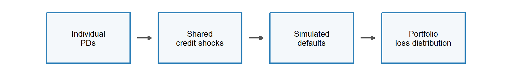
Figure 5.1: Gaussian copula workflow for portfolio credit risk.

The workflow separates marginal default risk, co-default behavior, and loss severity. Marginal default risk describes each firm one at a time, before adding common shocks across firms. For firm $i$, the cumulative default probability $Q_i(T)$ is the probability that the firm has defaulted at some point between today and horizon $T$. It accumulates default risk over the interval from 0 to $T$, so a 5-year cumulative PD includes defaults that occur in years 1, 2, 3, 4, or 5.

Co-default behavior enters through the copula correlation $\rho$. The parameter $\rho$ controls how strongly the firms’ credit-state scores share common shocks. When $\rho$ is higher, weak credit states tend to arrive for several firms in the same scenario. Lower values of the credit-state score mean weaker credit conditions, and default occurs when the score falls below its threshold. Loss severity comes from exposures and recoveries. After defaults are simulated, exposures and recoveries convert each default event into a money loss.

This separation is why copulas are useful in credit risk. We can hold each firm’s default probability fixed and change the common-shock correlation. When the tail of the loss distribution changes, joint default behavior drives that change.

Code

kable(
  copula_input_table,
  caption = "Objects used in the Gaussian copula credit-risk workflow.",
  escape = FALSE
)

Objects used in the Gaussian copula credit-risk workflow.
Object	Code	Financial role
$Q_i(T)$	`pd_cum`	Cumulative default probability of firm $i$ by horizon $T$.
$X_i$	simulated standard normal credit-state score	Model score summarizing firm $i$’s credit condition in a scenario; lower values mean weaker credit.
$z_i(T)=N^{-1}(Q_i(T))$	`default_threshold <- qnorm(pd_cum)`	Default threshold; values below this boundary are defaults.
$\rho$	`rho`	Correlation between credit-state scores before converting them into 0/1 defaults.
$EAD_i$	`ead`	Exposure at default measuring the amount at risk.
$R_i$	`recovery`	Fraction recovered after default.
$LGD_i=1-R_i$	`lgd <- 1 - recovery`	Fraction lost after default.

One detail is worth making explicit before we code. In the Gaussian copula simulation, $\rho$ is the correlation between the standardized normal credit-state scores $X_i$ and $X_j$. These are the continuous credit states we simulate first.

The binary default variable $Y_i(T)$ is created after the threshold rule is applied. It equals 1 when firm $i$ defaults by horizon $T$ and 0 otherwise. We use $Y_i(T)$ here to avoid confusing the default indicator with the promised debt payment $D$ from the Merton chapter. The sample correlation between $Y_i(T)$ and $Y_j(T)$ is therefore a result of the simulation, and it depends on both $\rho$ and the default thresholds. Later in the chapter we compute joint default probabilities directly from the simulated defaults.

We now need one bridge between a default probability and a simulation rule. The bridge is a default threshold. Suppose firm $i$ has cumulative probability of default $Q_i(T)$ by horizon $T$. The Gaussian copula represents the firm’s credit state with a standard normal score $X_i$. The threshold is the point on the normal scale that leaves probability $Q_i(T)$ to its left:

\[ z_i(T)=N^{-1}(Q_i(T)). \]

The simulation rule is then

\[ \text{firm } i \text{ defaults by } T \quad \Longleftrightarrow \quad X_i \leq z_i(T). \]

The rule preserves the marginal default probability by construction. The inverse normal function $N^{-1}(\cdot)$ finds the value whose left-tail area is exactly $Q_i(T)$, so the probability of falling below the threshold is the original cumulative PD.

\[ P(X_i \leq z_i(T))=P(X_i \leq N^{-1}(Q_i(T)))=Q_i(T). \]

For the 5-year PD used below, pd_cum[5] is 15.0%. The threshold is -1.0364, obtained with qnorm(pd_cum[5]). A simulated value of $X_i$ below -1.0364 is counted as a default by year 5. Since pnorm(default_threshold[5]) returns 15.0%, the threshold check recovers the same cumulative PD.

This is why the code uses the pair qnorm() and pnorm(). The function qnorm() translates a cumulative PD into a normal threshold. The function pnorm() is the check that the threshold reproduces the same cumulative PD.

5.2 Hull Example 24.7 from cumulative PDs to thresholds

The example that belongs to this chapter is Hull’s Example 24.7. The example immediately before it, Example 24.6, is about CVA for a gold forward contract. The Gaussian-copula credit portfolio example starts after Hull motivates default correlation in section 24.8.

Hull’s Example 24.7 considers ten firms. Each firm has the same cumulative probabilities of default over five horizons.

In this example, the cumulative PDs are inputs. In practice, they would have to be estimated before using the copula. They could come from an internal credit-scoring model like the models in Chapters 1 and 2, from a structural model such as Merton for public firms, from historical default rates for comparable rating or industry groups, or from market-implied credit information. The copula starts after these marginal PDs are available. Its job is to combine the individual default probabilities with a dependence assumption so we can simulate which firms default together.

\[ Q(1)=1\%,\quad Q(2)=3\%,\quad Q(3)=6\%,\quad Q(4)=10\%,\quad Q(5)=15\%. \]

The word cumulative is important. A cumulative 5-year PD of 15% means default occurs sometime between today and year 5. A separate 15% default probability inside year 5 would describe a different object. The incremental probability for a specific year is obtained by differencing the cumulative curve. For example, the probability of default between year 4 and year 5 is

\[ Q(5)-Q(4)=15\%-10\%=5\%. \]

The table below keeps both objects visible because they answer different questions. The cumulative PD is used to define the default threshold by horizon. The incremental PD tells us how much new default probability is added between two adjacent horizons. The last column is a check. It applies $N(\cdot)$ back to the threshold, so it should reproduce the cumulative PD exactly apart from rounding. In other words, the cumulative PD is the input, the default threshold is the normal-scale version of that input, and the recovered PD confirms that the transformation preserves the marginal default probability.

Code

kable(
  hull_threshold_table,
  caption = "Hull Example 24.7 inputs and the corresponding Gaussian default thresholds.",
  escape = FALSE
)

Hull Example 24.7 inputs and the corresponding Gaussian default thresholds.
Horizon	Cumulative PD	Incremental PD	Default threshold	PD recovered from threshold
1 year	1.00%	1.00%	-2.326348	1.00%
2 years	3.00%	2.00%	-1.880794	3.00%
3 years	6.00%	3.00%	-1.554774	6.00%
4 years	10.00%	4.00%	-1.281552	10.00%
5 years	15.00%	5.00%	-1.036433	15.00%

The code below shows the transformation and its check.

Code

pd_cum <- c(0.01, 0.03, 0.06, 0.10, 0.15)
default_threshold <- qnorm(pd_cum)
pnorm(default_threshold)

[1] 0.01 0.03 0.06 0.10 0.15

The financial meaning is longer than the code. pd_cum contains marginal cumulative default probabilities. The command qnorm(pd_cum) converts those probabilities into normal-scale default thresholds. The command pnorm(default_threshold) walks back from the threshold to the probability scale. It gives the same numerical values as pd_cum by construction, and that equality is useful because it proves that the threshold rule preserves the individual default probabilities before we link firms through shared shocks.

For the 5-year horizon, the threshold is -1.036433. A simulated firm defaults by year 5 if its credit-state score is below that value.

\[ Y_i(5)= \begin{cases} 1, & \text{if } X_i \leq -1.036433,\\ 0, & \text{if } X_i > -1.036433. \end{cases} \]

$Y_i(5)$ is therefore a binary default variable. It equals 1 when firm $i$ defaults by year 5 and equals 0 when the firm survives through year 5. The cutoff rule is simple: values of $X_i$ below the threshold are counted as defaults, and values above the threshold are counted as survival.

Because $X_i$ is standard normal, this rule gives

\[ P(Y_i(5)=1)=P(X_i \leq -1.036433)=N(-1.036433) = 15.00%. \]

A single simulated scenario can be read directly from the same rule. The next table uses the 5-year threshold and a few illustrative credit-state scores. A score below the threshold becomes $Y_i(5)=1$; a score above the threshold becomes $Y_i(5)=0$.

Code

threshold_scenario_example <- data.frame(
  Firm = c("Firm A", "Firm B", "Firm C", "Firm D"),
  Credit_state_score = c(-1.40, -1.05, -0.80, 0.25),
  Default_threshold = rep(default_threshold[5], 4)
)
threshold_scenario_example$`Y_i(5)` <- ifelse(
  threshold_scenario_example$Credit_state_score <=
    threshold_scenario_example$Default_threshold,
  1,
  0
)
threshold_scenario_example$Interpretation <- ifelse(
  threshold_scenario_example$`Y_i(5)` == 1,
  "Default by year 5",
  "Survival through year 5"
)

kable(
  transform(
    threshold_scenario_example,
    Credit_state_score = fmt_num(Credit_state_score, 2),
    Default_threshold = fmt_num(Default_threshold, 6)
  ),
  caption = "Illustrative threshold rule for one simulated credit scenario.",
  row.names = FALSE
)

Illustrative threshold rule for one simulated credit scenario.
Firm	Credit_state_score	Default_threshold	Y_i(5)	Interpretation
Firm A	-1.40	-1.036433	1	Default by year 5
Firm B	-1.05	-1.036433	1	Default by year 5
Firm C	-0.80	-1.036433	0	Survival through year 5
Firm D	0.25	-1.036433	0	Survival through year 5

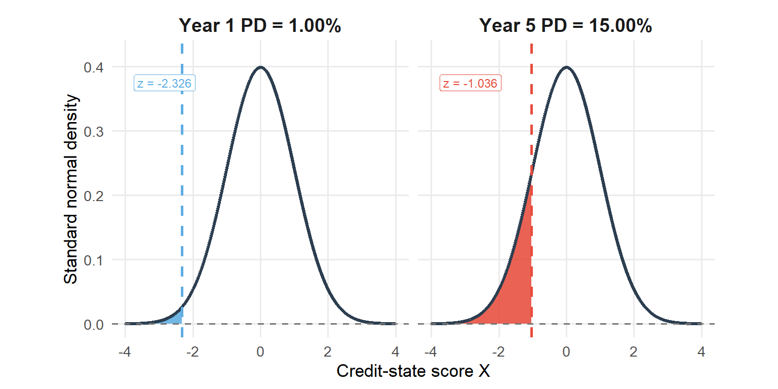
The figure below shows the same logic graphically for year 1 and year 5. The shaded area is the cumulative probability of default by that horizon.

Code

threshold_area_horizons <- c(1, 5)
threshold_area_labels <- paste0(
  "Year ", threshold_area_horizons,
  " PD = ", fmt_pct(pd_cum[threshold_area_horizons], 2)
)
threshold_area_colors <- c("#5DADE2", "#E74C3C")
names(threshold_area_colors) <- threshold_area_labels

threshold_area_data <- do.call(rbind, lapply(seq_along(threshold_area_horizons), function(j) {
  horizon_index <- threshold_area_horizons[j]
  data.frame(
    Horizon = threshold_area_labels[j],
    x = x,
    Density = D,
    Threshold = default_threshold[horizon_index],
    Shade = x <= default_threshold[horizon_index]
  )
}))
threshold_area_data$Horizon <- factor(threshold_area_data$Horizon, levels = threshold_area_labels)

threshold_label_data <- data.frame(
  Horizon = factor(threshold_area_labels, levels = threshold_area_labels),
  x = -3.75,
  y = 0.375,
  label = paste0("z = ", fmt_num(default_threshold[threshold_area_horizons], 3))
)

ggplot(threshold_area_data, aes(x = x, y = Density)) +
  geom_area(
    data = subset(threshold_area_data, Shade),
    aes(fill = Horizon),
    alpha = 0.88
  ) +
  geom_line(linewidth = 1.1, color = "#2C3E50") +
  geom_hline(yintercept = 0, linetype = "dashed", color = "#777777") +
  geom_vline(
    aes(xintercept = Threshold, color = Horizon),
    linetype = "dashed",
    linewidth = 0.9
  ) +
  geom_label(
    data = threshold_label_data,
    aes(x = x, y = y, label = label, color = Horizon),
    inherit.aes = FALSE,
    hjust = 0,
    size = 3.1,
    label.size = 0.2,
    fill = "white"
  ) +
  facet_wrap(~Horizon, nrow = 1) +
  scale_fill_manual(values = threshold_area_colors, guide = "none") +
  scale_color_manual(values = threshold_area_colors, guide = "none") +
  coord_cartesian(xlim = c(-4, 4), ylim = c(0, 0.42)) +
  labs(
    x = "Credit-state score X",
    y = "Standard normal density"
  ) +
  theme_minimal(base_size = 13) +
  theme(
    aspect.ratio = 1,
    strip.text = element_text(face = "bold", size = 14),
    panel.grid.minor = element_blank()
  )

Figure 5.2: Default thresholds implied by Hull Example 24.7 cumulative PDs.

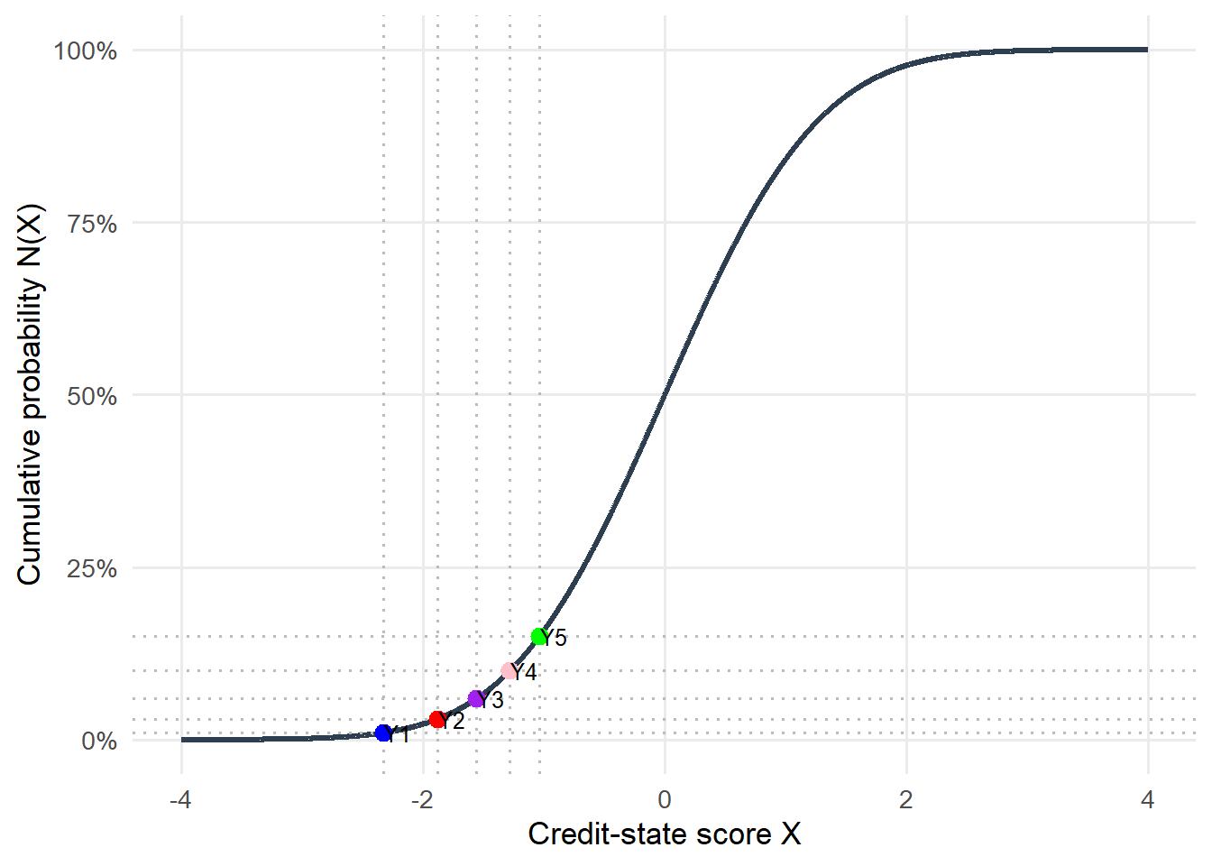
A second view uses the cumulative normal distribution directly. In this graph, the vertical axis already is the cumulative probability. The points show that each default threshold maps back to the PD input that produced it.

Code

threshold_curve_data <- data.frame(x = x, Probability = P)
threshold_points <- data.frame(
  Threshold = default_threshold,
  Cumulative_PD = pd_cum,
  Horizon = paste0("Y", credit_horizons)
)

ggplot(threshold_curve_data, aes(x = x, y = Probability)) +
  geom_line(linewidth = 1.1, color = "#2C3E50") +
  geom_hline(data = threshold_points, aes(yintercept = Cumulative_PD), linetype = "dotted", color = "#BBBBBB") +
  geom_vline(data = threshold_points, aes(xintercept = Threshold), linetype = "dotted", color = "#BBBBBB") +
  geom_point(data = threshold_points, aes(x = Threshold, y = Cumulative_PD, color = Horizon), size = 3) +
  geom_text(data = threshold_points, aes(x = Threshold, y = Cumulative_PD, label = Horizon), nudge_x = 0.12, size = 3.4) +
  scale_color_manual(values = colors2, guide = "none") +
  scale_y_continuous(labels = function(x) fmt_pct(x, 0)) +
  labs(
    x = "Credit-state score X",
    y = "Cumulative probability N(X)"
  ) +
  theme_minimal(base_size = 13) +
  theme(panel.grid.minor = element_blank())

Figure 5.3: Checking that each Gaussian threshold reproduces the original cumulative PD.

A zoomed version makes the relevant threshold region easier to inspect.

Code

ggplot(threshold_curve_data, aes(x = x, y = Probability)) +
  geom_line(linewidth = 1.1, color = "#2C3E50") +
  geom_hline(data = threshold_points, aes(yintercept = Cumulative_PD), linetype = "dotted", color = "#BBBBBB") +
  geom_vline(data = threshold_points, aes(xintercept = Threshold), linetype = "dotted", color = "#BBBBBB") +
  geom_point(data = threshold_points, aes(x = Threshold, y = Cumulative_PD, color = Horizon), size = 3.4) +
  geom_text(data = threshold_points, aes(x = Threshold, y = Cumulative_PD, label = Horizon), nudge_x = 0.04, size = 3.5) +
  scale_color_manual(values = colors2, guide = "none") +
  scale_y_continuous(labels = function(x) fmt_pct(x, 0)) +
  coord_cartesian(xlim = c(-2.5, -0.5), ylim = c(0, 0.2)) +
  labs(
    x = "Credit-state score X",
    y = "Cumulative probability N(X)"
  ) +
  theme_minimal(base_size = 13) +
  theme(panel.grid.minor = element_blank())

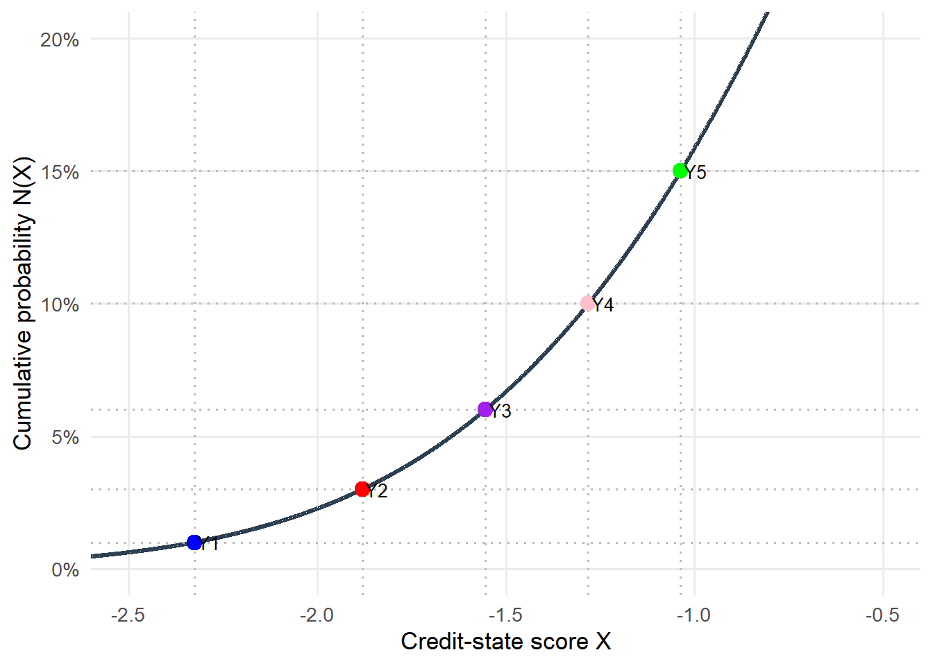
Figure 5.4: Zoom: Gaussian thresholds and cumulative PDs between -2.5 and -0.5.

At this stage, the chapter has built marginal default rules for each firm. The next step draws several credit-state scores in the same scenario. Independent draws represent borrowers whose credit states move separately. Correlated draws represent borrowers exposed to shared shocks. With a common copula correlation of 0.2, the probability of joint defaults changes while the individual PDs shown in this section are preserved.

5.3 One firm and the marginal default rule

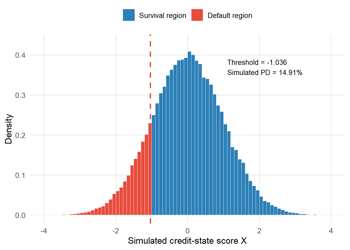
Before linking firms through common shocks, it is useful to check the one-firm rule. For the 5-year horizon in Hull’s Example 24.7, the cumulative PD is 15.00% and the default threshold is -1.036433.

The rule can be written as a two-case definition:

\[ Y_i(5)= \begin{cases} 1, & \text{if } X_i \leq N^{-1}(0.15),\\ 0, & \text{if } X_i > N^{-1}(0.15). \end{cases} \]

The R code applies the same rule.

Code

one_firm_sims <- 100000
one_firm_threshold <- qnorm(0.15)

set.seed(130575)
one_firm_x <- rnorm(one_firm_sims)
one_firm_default <- one_firm_x <= one_firm_threshold
one_firm_simulated_pd_from_code <- mean(one_firm_default)

The object one_firm_default is a TRUE/FALSE vector. R treats TRUE as 1 and FALSE as 0 when it computes a mean, so mean(one_firm_default) is the fraction of simulations in which the firm defaults.

With a finite number of random draws, the simulated PD lands close to 15.00%. That is the first sanity check. The simulation rule preserves the marginal PD before we link this firm to other firms.

Code

kable(
  one_firm_check,
  caption = "One-firm simulation check for the 5-year marginal PD.",
  escape = FALSE
)

One-firm simulation check for the 5-year marginal PD.
Horizon	Input PD	Default threshold	Simulated PD	Difference
5 years	15.00%	-1.036433	14.91%	-0.09%

In the figure, each simulated value of $X_i$ is a possible credit state for the firm. Lower values are weaker credit states. The firm defaults by year 5 when the simulated value falls to the left of the threshold.

Code

one_firm_hist <- hist(
  one_firm_x,
  breaks = 80,
  probability = TRUE,
  plot = FALSE
)
one_firm_hist_data <- data.frame(
  x_mid = one_firm_hist$mids,
  density = one_firm_hist$density,
  default_region = one_firm_hist$mids <= one_firm_threshold
)

ggplot(one_firm_hist_data, aes(x = x_mid, y = density, fill = default_region)) +
  geom_col(width = diff(one_firm_hist$breaks)[1], color = "white", linewidth = 0.1) +
  geom_vline(xintercept = one_firm_threshold, linewidth = 1, linetype = "dashed", color = "#E74C3C") +
  annotate(
    "label",
    x = 1.05,
    y = 0.37,
    hjust = 0,
    label = paste0(
      "Threshold = ", fmt_num(one_firm_threshold, 3),
      "\nSimulated PD = ", fmt_pct(one_firm_sim_pd, 2)
    ),
    size = 3.5,
    fill = "white",
    label.size = 0,
    linewidth = 0
  ) +
  scale_fill_manual(
    values = c("FALSE" = "#2C7FB8", "TRUE" = "#E74C3C"),
    labels = c("Survival region", "Default region"),
    name = NULL
  ) +
  coord_cartesian(xlim = c(-4, 4), ylim = c(0, 0.43)) +
  labs(
    x = "Simulated credit-state score X",
    y = "Density"
  ) +
  theme_minimal(base_size = 13) +
  theme(
    legend.position = "top",
    panel.grid.minor = element_blank()
  )

Figure 5.5: One-firm simulation check with threshold comparison.

This one-firm check verifies the marginal default mechanism. The copula model begins when we draw several firms’ credit-state scores in the same scenario and let shared shocks make those scores correlated.

5.4 Two firms and joint defaults

The two-firm case shows what the copula adds. Suppose both firms have the same 5-year cumulative PD, 15.00%. If the two default events were independent, the probability that both default by year 5 would be

\[ P(A\text{ defaults and }B\text{ defaults}) =15.00%\times 15.00% =2.25%. \]

The probability that at least one defaults would be

\[ P(A\text{ or }B\text{ defaults}) =1-(1-15.00%)^2 =27.75%. \]

Those formulas rely on independence. Under independence, firm A’s credit state and firm B’s credit state are unrelated. The Gaussian copula adds shared shocks, so low values of $X_A$ and $X_B$ can occur together more often while each firm keeps a marginal PD near 15.00%.

The covariance matrix tells R how strongly the two credit-state scores share shocks.

\[ \Sigma= \begin{bmatrix} 1 & \rho\\ \rho & 1 \end{bmatrix}. \]

Code

rho <- 0.2
sigma <- matrix(c(1, rho, rho, 1), nrow = 2)

set.seed(130575)
credit_state <- MASS::mvrnorm(
  n = 100000,
  mu = c(0, 0),
  Sigma = sigma
)

threshold <- qnorm(0.15)
default_a <- credit_state[, 1] <= threshold
default_b <- credit_state[, 2] <= threshold

two_firm_direct_check <- data.frame(
  Quantity = c(
    "Simulated PD for firm A",
    "Simulated PD for firm B",
    "Simulated joint-default probability"
  ),
  Value = c(
    fmt_pct(mean(default_a), 2),
    fmt_pct(mean(default_b), 2),
    fmt_pct(mean(default_a & default_b), 2)
  )
)

knitr::kable(
  two_firm_direct_check,
  caption = "Direct two-firm simulation check for rho = 0.2.",
  row.names = FALSE
)

Direct two-firm simulation check for rho = 0.2.
Quantity	Value
Simulated PD for firm A	15.02%
Simulated PD for firm B	14.88%
Simulated joint-default probability	3.44%

The first two probabilities check the marginal PDs. The third probability is the joint default probability. That is where the shared-shock assumption becomes visible.

Code

kable(
  two_firm_table,
  caption = "Two-firm default probabilities under different Gaussian copula correlations.",
  escape = FALSE
)

Two-firm default probabilities under different Gaussian copula correlations.
rho	PD A	PD B	P(A and B)	P(A or B)	Default corr.
-0.5	15.05%	14.92%	0.31%	29.66%	-0.1521
-0.2	15.02%	15.02%	1.28%	28.76%	-0.0762
0.0	14.94%	14.91%	2.19%	27.66%	-0.0030
0.2	15.02%	14.88%	3.44%	26.46%	0.0948
0.5	14.92%	14.94%	5.73%	24.13%	0.2754

The table demonstrates the main point. The marginal PDs stay close to 15.00%, while the probability of both firms defaulting rises as $\rho$ rises. Negative correlation pushes joint defaults down, positive correlation pushes them up, and $\rho=0$ gives the independent benchmark. The default-variable correlation is lower than the correlation between credit-state scores because default is a tail event created after applying the threshold.

The union probability also helps explain what correlation changes. For two firms,

\[ P(A \text{ or } B)=P(A)+P(B)-P(A \text{ and } B). \]

The marginal probabilities $P(A)$ and $P(B)$ remain close to 15.00%. As $\rho$ moves from 0 to 0.5, the simulated joint-default probability rises from 2.19% to 5.73%. Because the joint-default term is subtracted in the union formula, the probability that at least one firm defaults falls from 27.66% to 24.13%. Higher correlation moves defaults into the same scenarios.

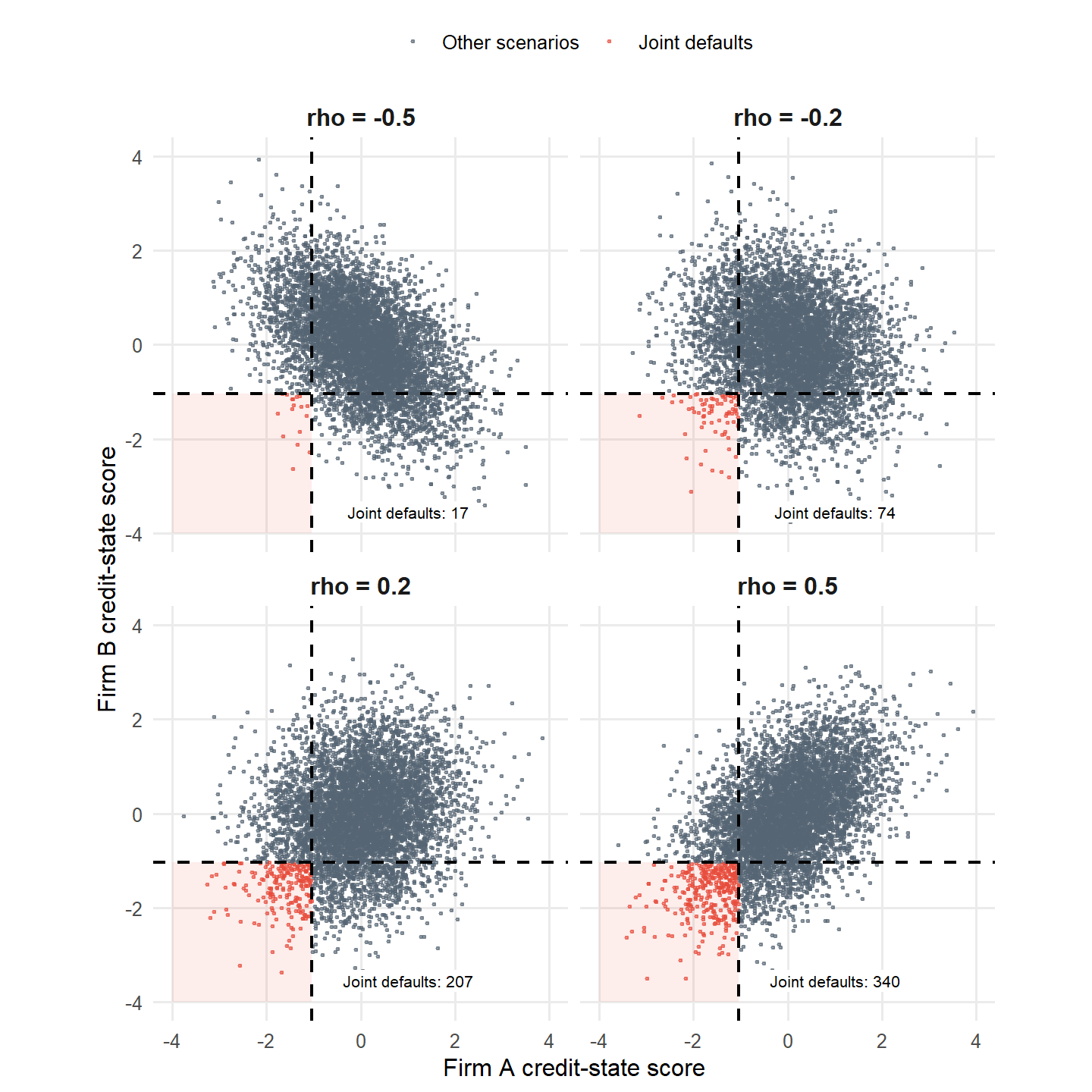
The scatter plots show the same mechanism and widen the comparison to negative and positive correlations. Each dot is one simulated pair $(X_A,X_B)$, meaning one credit scenario for the two firms. A firm defaults when its credit-state score is below the threshold. The lower-left region is the joint-default region. Negative correlations are included here because the two-firm case can support them and they make the mechanics visible. Positive correlation makes weak credit states arrive together more often.

The negative-correlation panels are useful for learning because they show the opposite of default clustering. In larger portfolio applications, the correlation matrix must remain internally consistent, and credit portfolios are usually dominated by positive common shocks such as recessions, sector stress, and funding pressure. For that reason, the portfolio sections focus on nonnegative dependence.

Code

two_firm_scatter_data <- do.call(rbind, lapply(two_firm_plot_data, function(plot_data) {
  rho <- unique(plot_data$rho)
  rho_label <- paste0("rho = ", fmt_num(rho, 1))
  data.frame(
    firm_a = plot_data$firm_a,
    firm_b = plot_data$firm_b,
    rho = rho,
    rho_label = rho_label,
    joint_default = plot_data$firm_a <= two_firm_threshold &
      plot_data$firm_b <= two_firm_threshold
  )
}))
two_firm_scatter_data$rho_label <- factor(
  two_firm_scatter_data$rho_label,
  levels = paste0("rho = ", fmt_num(two_firm_plot_layout_rhos, 1))
)
two_firm_panel_data <- unique(
  two_firm_scatter_data[, c("rho", "rho_label")]
)
two_firm_joint_counts <- aggregate(
  joint_default ~ rho_label,
  data = two_firm_scatter_data,
  FUN = sum
)
two_firm_joint_counts$label <- paste0("Joint defaults: ", fmt_int(two_firm_joint_counts$joint_default))

ggplot(two_firm_scatter_data, aes(x = firm_a, y = firm_b)) +
  geom_rect(
    data = two_firm_panel_data,
    aes(xmin = -4, xmax = two_firm_threshold, ymin = -4, ymax = two_firm_threshold),
    inherit.aes = FALSE,
    fill = "#E74C3C",
    alpha = 0.10
  ) +
  geom_point(aes(color = joint_default), size = 0.45, alpha = 0.55) +
  geom_vline(xintercept = two_firm_threshold, linetype = "dashed", linewidth = 0.8) +
  geom_hline(yintercept = two_firm_threshold, linetype = "dashed", linewidth = 0.8) +
  geom_label(
    data = two_firm_joint_counts,
    aes(x = 1.0, y = -3.55, label = label),
    inherit.aes = FALSE,
    size = 2.8,
    fill = "white",
    label.size = 0,
    linewidth = 0
  ) +
  facet_wrap(~rho_label, ncol = 2) +
  scale_color_manual(
    values = c("FALSE" = adjustcolor("#566573", alpha.f = 0.55), "TRUE" = "#E74C3C"),
    labels = c("Other scenarios", "Joint defaults"),
    name = NULL
  ) +
  coord_equal(xlim = c(-4, 4), ylim = c(-4, 4)) +
  labs(
    x = "Firm A credit-state score",
    y = "Firm B credit-state score"
  ) +
  theme_minimal(base_size = 12) +
  theme(
    legend.position = "top",
    legend.background = element_rect(fill = "white", color = NA),
    legend.key = element_rect(fill = "white", color = NA),
    strip.text = element_text(face = "bold", size = 12),
    strip.background = element_rect(fill = "white", color = NA),
    panel.grid.minor = element_blank()
  )

Figure 5.6: Two-firm Gaussian copula simulations across negative and positive correlations.

This first credit-risk application of the copula separates the individual default probability of each firm from the co-default pattern between firms. The PD of each firm stays fixed, while the probability of clustered defaults changes.

5.5 Ten firms in the Hull portfolio default simulation

Hull’s Example 24.7 moves from three ingredients to a portfolio simulation. The ingredients are ten firms, the same cumulative PD curve for every firm, and a common copula correlation of 0.2 between every pair of credit-state scores.

The correlation matrix is therefore exchangeable.

\[ \Sigma_{ii}=1,\qquad \Sigma_{ij}=\rho \quad \text{for } i\neq j. \]

The R code creates the matrix.

Code

n_firms_hull <- 10
rho <- 0.2

sigma <- matrix(rho, nrow = n_firms_hull, ncol = n_firms_hull)
diag(sigma) <- 1
kable(
  sigma,
  digits = 1,
  caption = "Exchangeable correlation matrix for Hull Example 24.7."
)

Exchangeable correlation matrix for Hull Example 24.7.
1.0	0.2	0.2	0.2	0.2	0.2	0.2	0.2	0.2	0.2
0.2	1.0	0.2	0.2	0.2	0.2	0.2	0.2	0.2	0.2
0.2	0.2	1.0	0.2	0.2	0.2	0.2	0.2	0.2	0.2
0.2	0.2	0.2	1.0	0.2	0.2	0.2	0.2	0.2	0.2
0.2	0.2	0.2	0.2	1.0	0.2	0.2	0.2	0.2	0.2
0.2	0.2	0.2	0.2	0.2	1.0	0.2	0.2	0.2	0.2
0.2	0.2	0.2	0.2	0.2	0.2	1.0	0.2	0.2	0.2
0.2	0.2	0.2	0.2	0.2	0.2	0.2	1.0	0.2	0.2
0.2	0.2	0.2	0.2	0.2	0.2	0.2	0.2	1.0	0.2
0.2	0.2	0.2	0.2	0.2	0.2	0.2	0.2	0.2	1.0

The simulation then creates one row per scenario and one column per firm. Each cell is a simulated credit-state score. The threshold rule converts those scores into defaults.

Code

portfolio_sims <- 100000

set.seed(130575)
credit_state <- MASS::mvrnorm(
  n = portfolio_sims,
  mu = rep(0, n_firms_hull),
  Sigma = sigma
)

threshold_5y <- qnorm(0.15)
defaults_5y <- credit_state <= threshold_5y
default_count_5y <- rowSums(defaults_5y)
head(default_count_5y)

[1] 0 0 1 3 2 4

The object defaults_5y is the key credit-risk object. It is a matrix of TRUE/FALSE binary default variables. A row is one simulated credit scenario. A column is one firm. The sum across a row is the number of defaults in that portfolio scenario.

For the Hull correlation case $\rho=0.2$, the simulated distribution of the number of defaults by year 5 is shown below.

Code

hull_distribution_table <- data.frame(
  Defaults = hull_distribution$Defaults,
  Frequency = fmt_int(hull_distribution$Frequency),
  Probability = fmt_pct(hull_distribution$Probability, 3)
)

kable(
  hull_distribution_table,
  caption = "Distribution of the number of defaults by year 5 for ten firms and rho = 0.2.",
  escape = FALSE
)

Distribution of the number of defaults by year 5 for ten firms and rho = 0.2.
Defaults	Frequency	Probability
0	31,782	31.782%
1	27,767	27.767%
2	18,302	18.302%
3	11,029	11.029%
4	5,949	5.949%
5	3,021	3.021%
6	1,336	1.336%
7	558	0.558%
8	197	0.197%
9	54	0.054%
10	5	0.005%

This table gives more information than the individual PD. The 5-year PD of each firm is still 15.00%, while the portfolio manager also sees the probability of no defaults, one default, several defaults, and a cluster of defaults.

The next table compares different common-shock correlations while keeping the individual PD fixed.

Code

kable(
  event_summary_table,
  caption = "Default-event probabilities for ten firms under different copula correlations.",
  row.names = FALSE,
  escape = FALSE
)

Default-event probabilities for ten firms under different copula correlations.
rho	E[defaults]	P(0)	P(>=1)	P(>=3)	P(>=5)	P(10)
0.0	1.502	19.62%	80.38%	18.03%	0.96%	0.0000%
0.2	1.504	31.78%	68.22%	22.15%	5.17%	0.0050%
0.5	1.503	47.73%	52.27%	22.77%	10.59%	0.4590%

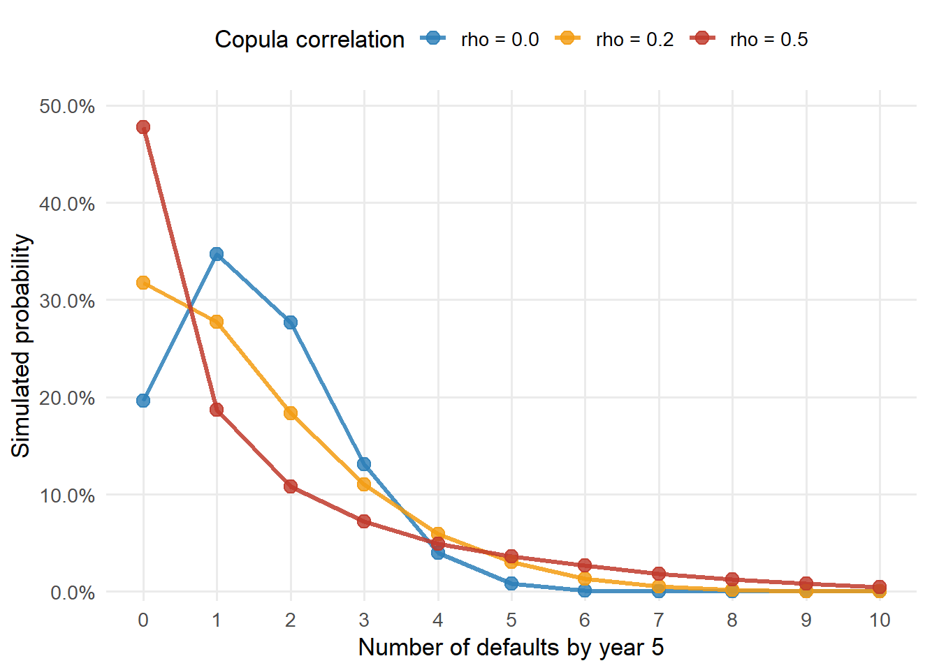
In the table, $P(\ge k)$ means the probability of $k$ or more defaults by year 5.

The expected number of defaults is close to 1.50 in every scenario because each firm still has a 15.00% marginal PD:

\[ E[N_{\text{defaults}}] =P(Y_1(5)=1)+\cdots+P(Y_{10}(5)=1) =10\times 0.15 =1.50. \]

Linearity of expectation gives the same average under independence, weak correlation, or high correlation. Correlation changes the shape of the distribution. Higher correlation increases the probability of very quiet portfolios and also the probability of severe default clusters. It reduces the middle cases where diversification works smoothly.

Code

default_counts <- 0:n_firms_hull
default_count_colors <- c("#2C7FB8", "#F39C12", "#C0392B")
default_count_plot_data <- data.frame(
  Defaults = rep(default_counts, times = ncol(count_probability_matrix)),
  Probability = as.vector(count_probability_matrix),
  Correlation = factor(
    rep(colnames(count_probability_matrix), each = length(default_counts)),
    levels = colnames(count_probability_matrix)
  )
)

ggplot(
  default_count_plot_data,
  aes(x = Defaults, y = Probability, color = Correlation, group = Correlation)
) +
  geom_line(linewidth = 1.1, alpha = 0.85) +
  geom_point(size = 3.2, alpha = 0.82) +
  scale_color_manual(values = default_count_colors) +
  scale_x_continuous(breaks = default_counts) +
  scale_y_continuous(
    labels = function(x) fmt_pct(x, 1),
    expand = expansion(mult = c(0.02, 0.08))
  ) +
  labs(
    x = "Number of defaults by year 5",
    y = "Simulated probability",
    color = "Copula correlation"
  ) +
  theme_minimal(base_size = 13) +
  theme(
    legend.position = "top",
    panel.grid.minor = element_blank(),
    plot.margin = margin(5.5, 12, 5.5, 5.5)
  )

Figure 5.7: Distribution of the number of defaults by year 5 under different copula correlations.

This is the main lesson of the Gaussian copula in a portfolio. Individual PDs determine the average default rate. The common-shock correlation determines how much probability mass moves into joint-default states.

5.6 From correlated defaults to portfolio losses

Defaults become financially useful when we attach exposures and recoveries. In one simulated credit scenario $s$, portfolio loss is

\[ L_s=\sum_{i=1}^n EAD_i \times LGD_i \times Y_{i,s}, \]

where $Y_{i,s}$ equals 1 when firm $i$ defaults in scenario $s$ and 0 otherwise. The code applies the same calculation.

Code

ead <- rep(10e6, 10)
recovery <- rep(0.40, 10)
lgd <- 1 - recovery

losses <- defaults_5y %*% (ead * lgd)

The example below uses a homogeneous portfolio with 10 firms, total exposure of $100 million, $10 million exposure per firm, 40% recovery, and a 5-year cumulative PD of 15.00% for every firm. The recovery assumption implies an LGD of 60%.

Expected loss can be understood before running the portfolio scenarios.

\[ EL = \sum_{i=1}^{10} EAD_i \times LGD_i \times PD_i = 10 \times 10{,}000{,}000 \times 0.60 \times 0.15 \]

The last expression is 9.00 million dollars.

The simulation should produce an expected loss close to that value in every correlation scenario, because the threshold rule keeps each firm’s marginal PD fixed. The tail of the loss distribution is the object that changes when shared shocks make default clusters more or less likely.

Code

kable(
  loss_summary_table,
  caption = "Portfolio loss summary for a homogeneous ten-firm portfolio.",
  escape = FALSE
)

Portfolio loss summary for a homogeneous ten-firm portfolio.
rho	EL	Median	VaR 95%	VaR 99%	VaR 99.9%	ES 99%	Capital 99.9%
0.0	$9.01m	$6.00m	$18.00m	$24.00m	$36.00m	$25.36m	$26.99m
0.2	$9.02m	$6.00m	$30.00m	$36.00m	$48.00m	$39.16m	$38.98m
0.5	$9.02m	$6.00m	$36.00m	$54.00m	$60.00m	$56.15m	$50.98m

The table separates three ideas. Expected loss is the average credit cost implied by PD, EAD, and LGD. VaR is a high percentile of the simulated loss distribution. Economic capital is the difference between a tail loss measure and expected loss.

For the Hull correlation case $\rho=0.2$, the expected loss is $9.02m, while the 99.9% VaR is $48.00m. The economic-capital number, $38.98m, is the extra loss buffer above expected loss at that confidence level. This is the practical reason the tail can dominate capital needs: two portfolios can have similar expected loss and very different capital buffers.

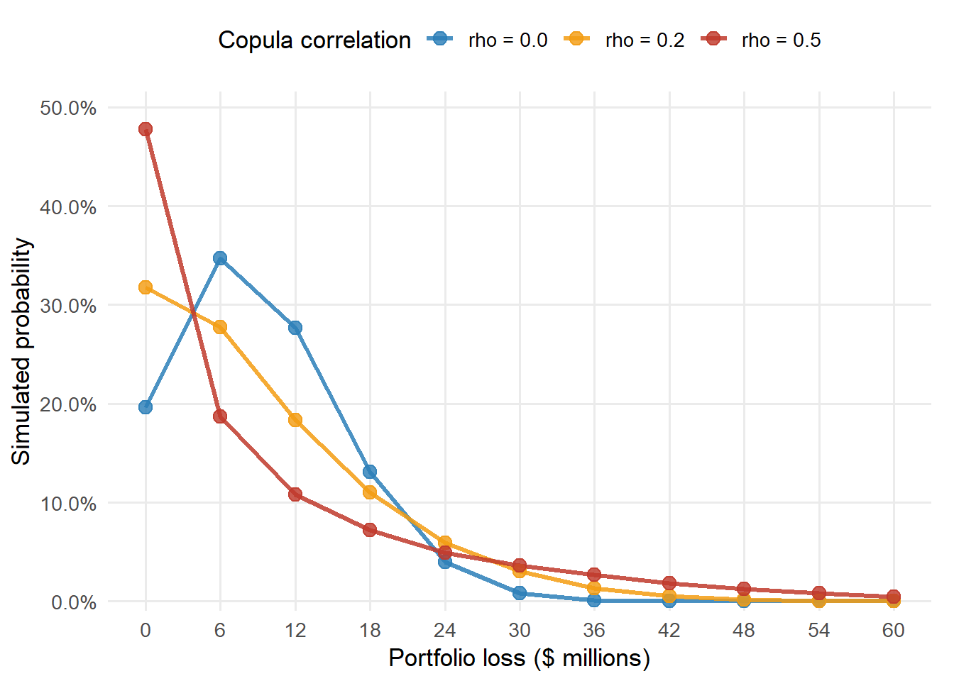
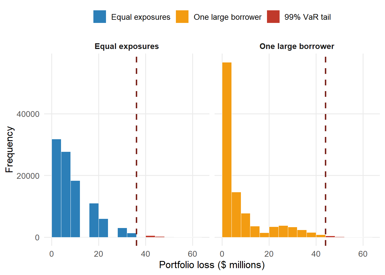
The next figure shows the simulated loss distribution. Because the portfolio has equal exposures and equal recoveries, losses occur in steps of $6 million per default.

Code

loss_steps <- 0:loss_n_firms
loss_distribution_colors <- c("#2C7FB8", "#F39C12", "#C0392B")
loss_distribution_plot_data <- data.frame(
  Loss = rep(loss_steps * loss_ead[1] * loss_lgd[1] / 1e6, times = ncol(loss_distribution_matrix)),
  Probability = as.vector(loss_distribution_matrix),
  Correlation = factor(
    rep(colnames(loss_distribution_matrix), each = length(loss_steps)),
    levels = colnames(loss_distribution_matrix)
  )
)

ggplot(
  loss_distribution_plot_data,
  aes(x = Loss, y = Probability, color = Correlation, group = Correlation)
) +
  geom_line(linewidth = 1.1, alpha = 0.85) +
  geom_point(size = 3.2, alpha = 0.82) +
  scale_color_manual(values = loss_distribution_colors) +
  scale_x_continuous(breaks = loss_steps * loss_ead[1] * loss_lgd[1] / 1e6) +
  scale_y_continuous(
    labels = function(x) fmt_pct(x, 1),
    expand = expansion(mult = c(0.02, 0.08))
  ) +
  labs(
    x = "Portfolio loss ($ millions)",
    y = "Simulated probability",
    color = "Copula correlation"
  ) +
  theme_minimal(base_size = 13) +
  theme(
    legend.position = "top",
    panel.grid.minor = element_blank(),
    plot.margin = margin(5.5, 12, 5.5, 5.5)
  )

Figure 5.8: Portfolio loss distribution under different copula correlations.

This is where the copula becomes a credit-risk tool. The marginal PD tells us the average loss. The common-shock correlation tells us how much probability sits in the severe-loss states.

5.7 Concentration risk with different exposure weights

The copula controls the co-default pattern. Portfolio loss also depends on exposure concentration. To isolate this point, keep the same simulated default matrix, the same PDs, the same recovery rate, the same copula correlation, and the same total exposure. Change only the exposure weights.

Using the same default matrix means every row has the same firms defaulting in both portfolios. The experiment changes the dollar loss attached to those default events. This isolates exposure concentration from default frequency.

The comparison uses two portfolios.

Equal exposures with ten firms at $10 million each.
One large borrower with one firm at $40 million and nine firms sharing the remaining $60 million.

Both portfolios have $100 million of total EAD. Since all firms have the same PD and recovery, expected loss is almost the same. Tail loss becomes larger when the high-exposure borrower appears in severe default scenarios.

Code

kable(
  concentration_summary_table,
  caption = "Concentration risk with the same total exposure, PD, recovery, and copula correlation.",
  escape = FALSE
)

Concentration risk with the same total exposure, PD, recovery, and copula correlation.
Portfolio	Max EAD	EL	VaR 99%	VaR 99.9%	ES 99%	Capital 99.9%
Equal exposures	$10.00m	$9.02m	$36.00m	$48.00m	$39.16m	$38.98m
One large borrower	$40.00m	$9.03m	$44.00m	$52.00m	$46.46m	$42.97m

The reason is simple and important. In the equal-exposure portfolio, each default adds the same loss. In the concentrated portfolio, the default of the largest borrower creates a much larger loss jump. The default-count distribution stays the same, while the loss distribution changes.

Numerically, one default in the equal-exposure portfolio adds $6.00m of loss. The default of the largest borrower in the concentrated portfolio adds $24.00m. That larger jump raises 99.9% economic capital by $3.99m even though the total EAD, PDs, recoveries, and simulated default scenarios are held fixed.

Code

concentration_breaks <- seq(0, max(loss_concentrated) / 1e6 + 4, by = 4)
make_concentration_hist_data <- function(losses, var_value, portfolio) {
  hist_object <- hist(
    losses / 1e6,
    breaks = concentration_breaks,
    plot = FALSE
  )
  data.frame(
    Portfolio = portfolio,
    x_mid = hist_object$mids,
    Frequency = hist_object$counts,
    Tail = hist_object$mids >= var_value / 1e6
  )
}

concentration_hist_data <- rbind(
  make_concentration_hist_data(
    loss_equal,
    concentration_summary_numeric["Equal_exposures", "var_99"],
    "Equal exposures"
  ),
  make_concentration_hist_data(
    loss_concentrated,
    concentration_summary_numeric["Concentrated_exposure", "var_99"],
    "One large borrower"
  )
)
concentration_hist_data$Portfolio <- factor(
  concentration_hist_data$Portfolio,
  levels = c("Equal exposures", "One large borrower")
)
concentration_hist_data$Fill <- ifelse(
  concentration_hist_data$Tail,
  "99% VaR tail",
  as.character(concentration_hist_data$Portfolio)
)
concentration_var_data <- data.frame(
  Portfolio = factor(c("Equal exposures", "One large borrower"), levels = levels(concentration_hist_data$Portfolio)),
  VaR = c(
    concentration_summary_numeric["Equal_exposures", "var_99"],
    concentration_summary_numeric["Concentrated_exposure", "var_99"]
  ) / 1e6
)

ggplot(concentration_hist_data, aes(x = x_mid, y = Frequency, fill = Fill)) +
  geom_col(width = diff(concentration_breaks)[1], color = "white", linewidth = 0.15) +
  geom_vline(
    data = concentration_var_data,
    aes(xintercept = VaR),
    inherit.aes = FALSE,
    color = "#7B241C",
    linewidth = 1,
    linetype = "dashed"
  ) +
  facet_wrap(~Portfolio, nrow = 1) +
  scale_fill_manual(
    values = c(
      "Equal exposures" = "#2C7FB8",
      "One large borrower" = "#F39C12",
      "99% VaR tail" = "#C0392B"
    ),
    breaks = c("Equal exposures", "One large borrower", "99% VaR tail"),
    name = NULL
  ) +
  labs(
    x = "Portfolio loss ($ millions)",
    y = "Frequency"
  ) +
  theme_minimal(base_size = 13) +
  theme(
    legend.position = "top",
    strip.text = element_text(face = "bold"),
    panel.grid.minor = element_blank()
  )

Figure 5.9: Same defaults and different exposure weights.

This application moves from borrower-level PD to portfolio-level loss. A portfolio can have the same average credit quality and the same total exposure, while its tail-loss profile changes because the exposures are concentrated.

5.8 Tail dependence with a t-copula

The Gaussian copula uses normal credit-state scores. The correlation parameter makes weak credit states arrive together more often. The normal distribution controls how much probability sits in extreme credit states. A t-copula keeps the same threshold idea and changes the tail shape.

For the Gaussian copula, one convenient one-factor representation is

\[ X_i^{G}=\sqrt{\rho}\,Z_0+\sqrt{1-\rho}\,Z_i. \]

For the t-copula, use the same normal factor structure and divide by a random scale shock:

\[ X_i^{t}= \frac{\sqrt{\rho}\,Z_0+\sqrt{1-\rho}\,Z_i} {\sqrt{S/\nu}}, \qquad S\sim\chi^2_{\nu}. \]

The parameter $\nu$ is the number of degrees of freedom. Lower $\nu$ means heavier tails, so extreme credit states occur more often. The default threshold changes from $N^{-1}(PD)$ to $t_{\nu}^{-1}(PD)$, so each firm keeps the same marginal PD. In code, this is the move from qnorm(tcopula_pd) to qt(tcopula_pd, df = df).

The scale shock is shared by all firms in a scenario. When $S/\nu$ is small, the denominator is small and the scenario becomes more extreme for the whole portfolio. Negative credit shocks are pushed further into the left tail, which creates more scenarios where several firms cross their default thresholds together. The model therefore changes the clustering of defaults without changing the average PD assigned to each firm.

The code below builds the comparison. It keeps the same number of firms, PD, exposure, recovery, and correlation. Then it changes only the copula family and, for the t-copula, the degrees of freedom.

Code

simulate_t_copula_credit <- function(n_sims, n_firms, rho, df, seed = 130575) {
  set.seed(seed)
  gaussian_latent <- MASS::mvrnorm(
    n = n_sims,
    mu = rep(0, n_firms),
    Sigma = make_correlation_matrix(n_firms, rho)
  )
  scale_shock <- sqrt(rchisq(n_sims, df = df) / df)
  gaussian_latent / scale_shock
}

tcopula_sims <- 100000
tcopula_n_firms <- 10
tcopula_rho <- hull_example_247_rho
tcopula_pd <- pd_cum[5]
tcopula_total_ead <- 100e6
tcopula_ead <- rep(tcopula_total_ead / tcopula_n_firms, tcopula_n_firms)
tcopula_recovery <- rep(0.40, tcopula_n_firms)

tcopula_design <- data.frame(
  copula = c("Gaussian", "t-copula", "t-copula"),
  df = c(NA, 10, 4)
)

simulate_tail_dependence_case <- function(copula, df) {
  if (copula == "Gaussian") {
    latent <- simulate_latent_credit(
      n_sims = tcopula_sims,
      n_firms = tcopula_n_firms,
      rho = tcopula_rho,
      seed = 130575
    )
    threshold <- qnorm(tcopula_pd)
  } else {
    latent <- simulate_t_copula_credit(
      n_sims = tcopula_sims,
      n_firms = tcopula_n_firms,
      rho = tcopula_rho,
      df = df,
      seed = 130575
    )
    threshold <- qt(tcopula_pd, df = df)
  }

  defaults <- make_default_matrix(latent, threshold)
  losses <- portfolio_losses(defaults, tcopula_ead, tcopula_recovery)

  list(
    defaults = defaults,
    default_count = rowSums(defaults),
    losses = losses,
    events = summarize_default_events(defaults),
    loss_summary = loss_risk_summary(losses),
    mean_pd = mean(defaults)
  )
}

tcopula_results <- Map(
  simulate_tail_dependence_case,
  tcopula_design$copula,
  tcopula_design$df
)
names(tcopula_results) <- c("Gaussian", "t df = 10", "t df = 4")

tcopula_events <- do.call(rbind, lapply(tcopula_results, function(x) x$events))
tcopula_losses <- do.call(rbind, lapply(tcopula_results, function(x) x$loss_summary))

tcopula_df_label <- ifelse(is.na(tcopula_design$df), "-", fmt_int(tcopula_design$df))

tcopula_default_table <- data.frame(
  Copula = tcopula_design$copula,
  df = tcopula_df_label,
  Mean_PD = fmt_pct(sapply(tcopula_results, function(x) x$mean_pd), 2),
  Expected_defaults = fmt_num(tcopula_events[, "expected_defaults"], 3),
  P_three_or_more = fmt_pct(tcopula_events[, "three_or_more"], 2),
  P_five_or_more = fmt_pct(tcopula_events[, "five_or_more"], 2),
  P_all_ten = fmt_pct(tcopula_events[, "all_default"], 3)
)
names(tcopula_default_table) <- c(
  "Copula",
  "df",
  "Mean PD",
  "E[defaults]",
  "P(>=3)",
  "P(>=5)",
  "P(10)"
)

tcopula_loss_table <- data.frame(
  Copula = tcopula_design$copula,
  df = tcopula_df_label,
  EL = fmt_musd(tcopula_losses[, "expected_loss"]),
  VaR_99 = fmt_musd(tcopula_losses[, "var_99"]),
  VaR_99_9 = fmt_musd(tcopula_losses[, "var_999"]),
  ES_99_9 = fmt_musd(tcopula_losses[, "es_999"]),
  Capital_99_9 = fmt_musd(tcopula_losses[, "economic_capital_999"])
)
names(tcopula_loss_table) <- c(
  "Copula",
  "df",
  "EL",
  "VaR 99%",
  "VaR 99.9%",
  "ES 99.9%",
  "Capital 99.9%"
)

tcopula_count_matrix <- sapply(tcopula_results, function(x) {
  as.numeric(tabulate(x$default_count + 1, nbins = tcopula_n_firms + 1)) /
    tcopula_sims
})
colnames(tcopula_count_matrix) <- names(tcopula_results)

The comparison below keeps the 5-year PD at 15.00%, the copula correlation at 0.2, the same 10 firms, the same total exposure, and the same recovery rate. The only change is the copula tail shape.

Code

kable(
  tcopula_default_table,
  caption = "Default clustering under Gaussian and t-copulas.",
  row.names = FALSE,
  escape = FALSE
)

Default clustering under Gaussian and t-copulas.
Copula	df	Mean PD	E[defaults]	P(>=3)	P(>=5)	P(10)
Gaussian	-	15.04%	1.504	22.15%	5.17%	0.005%
t-copula	10	15.05%	1.505	22.45%	6.04%	0.013%
t-copula	4	15.05%	1.505	23.06%	7.25%	0.033%

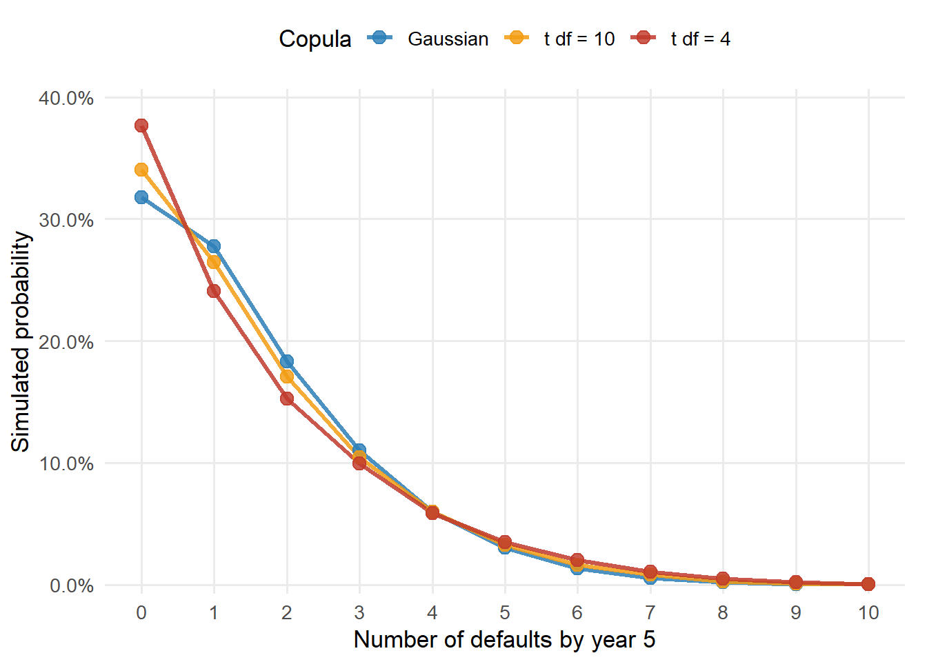
The average PD stays near 15.00%. The tail probabilities move because the t-copula gives more weight to scenarios where many firms experience weak credit states together. This is the credit-risk reason to care about tail dependence.

For example, the probability of five or more defaults rises from 5.17% under the Gaussian copula to 7.25% under the heavier-tailed t-copula. The probability that all ten firms default rises from 0.005% to 0.033%. The marginal PD remains anchored near 15%, so the difference is coming from joint-tail behavior.

The same default simulations can be translated into losses using the portfolio loss formula from the previous section.

Code

kable(
  tcopula_loss_table,
  caption = "Portfolio loss measures under Gaussian and t-copulas.",
  row.names = FALSE,
  escape = FALSE
)

Portfolio loss measures under Gaussian and t-copulas.
Copula	df	EL	VaR 99%	VaR 99.9%	ES 99.9%	Capital 99.9%
Gaussian	-	$9.02m	$36.00m	$48.00m	$49.50m	$38.98m
t-copula	10	$9.03m	$42.00m	$54.00m	$54.70m	$44.97m
t-copula	4	$9.03m	$42.00m	$54.00m	$54.95m	$44.97m

Expected loss remains anchored by PD, EAD, and LGD. Tail loss responds to the co-default model. This ten-firm portfolio has coarse $6 million loss steps, so VaR can land on the same step for two copulas. Expected shortfall is a useful companion because it averages the losses beyond the percentile.

Code

default_counts <- 0:tcopula_n_firms
tcopula_count_colors <- c("#2C7FB8", "#F39C12", "#C0392B")
tcopula_count_plot_data <- data.frame(
  Defaults = rep(default_counts, times = ncol(tcopula_count_matrix)),
  Probability = as.vector(tcopula_count_matrix),
  Copula = factor(
    rep(colnames(tcopula_count_matrix), each = length(default_counts)),
    levels = colnames(tcopula_count_matrix)
  )
)

ggplot(
  tcopula_count_plot_data,
  aes(x = Defaults, y = Probability, color = Copula, group = Copula)
) +
  geom_line(linewidth = 1.1, alpha = 0.85) +
  geom_point(size = 3.2, alpha = 0.82) +
  scale_color_manual(values = tcopula_count_colors) +
  scale_x_continuous(breaks = default_counts) +
  scale_y_continuous(
    labels = function(x) fmt_pct(x, 1),
    expand = expansion(mult = c(0.02, 0.08))
  ) +
  labs(
    x = "Number of defaults by year 5",
    y = "Simulated probability",
    color = "Copula"
  ) +
  theme_minimal(base_size = 13) +
  theme(
    legend.position = "top",
    panel.grid.minor = element_blank(),
    plot.margin = margin(5.5, 12, 5.5, 5.5)
  )

Figure 5.10: Default-count distribution under Gaussian and t-copulas.

This section gives the key model-risk message. A copula is more than a correlation input. It also chooses how much probability is assigned to joint tail events.

5.9 Credit VaR under copula model risk

The chapter now has all the pieces needed to make Credit VaR concrete. We have individual PDs, a co-default model, exposures, recoveries, a loss distribution, and tail-risk measures. Hull’s Credit VaR section, section 24.9 of (Hull 2022), gives a compact large-portfolio approximation.

The numerical setting changes in this section. Earlier we used Hull’s ten-firm, 5-year default example to learn how the copula creates co-default scenarios. Hull’s Credit VaR example uses a large homogeneous portfolio, a one-year PD of 2.00%, total exposure of $100.00m, recovery of 60.00%, and copula correlation of 0.10. The financial question also changes. We now ask how much capital is needed to absorb rare losses caused by a bad common credit factor.

The approximation applies to a large homogeneous portfolio. Each loan has the same one-year PD, the same recovery rate, and the same pairwise copula correlation. In a highly granular portfolio, borrower-specific noise largely diversifies away. Conditional on the common credit factor, the realized default fraction is close to the conditional default probability.

In the ten-firm simulations, the outcome was a default count from 0 to 10. In the large-portfolio approximation, the outcome is a default rate. Multiplying that rate by EAD and LGD turns the rate into a dollar loss.

The large-portfolio formula compresses the same one-factor logic into a percentile calculation. We use $\alpha$ for the confidence level, leaving $X_i$ for the credit-state score of firm $i$. The question is practical: when the common credit factor reaches the bad tail state associated with confidence level $\alpha$, what default rate would a highly diversified portfolio experience? That default rate is then multiplied by exposure and loss given default.

Under those assumptions, the tail default rate at confidence level $\alpha$ is

\[ V(\alpha,T)= N\left( \frac{N^{-1}(Q(T))+\sqrt{\rho}\,N^{-1}(\alpha)} {\sqrt{1-\rho}} \right). \]

The formula uses the same objects as the copula simulation. $Q(T)$ is the marginal cumulative PD. The parameter $\rho$ controls the strength of the common credit factor. The confidence level $\alpha$ selects how far into the bad tail we look. The output $V(\alpha,T)$ is Hull’s tail default-rate function for a large homogeneous portfolio. This is local Credit VaR notation; the asset-value notation $V_T$ in the Merton chapter referred to a different financial object.

The plus sign in the numerator comes from the bad state of the common credit factor. In the one-factor representation, low values of the common factor raise conditional default probabilities. The loss percentile at confidence level $\alpha$ corresponds to the factor quantile $N^{-1}(1-\alpha)$. Substituting that bad factor into the conditional PD formula gives the same expression as above because $-N^{-1}(1-\alpha)=N^{-1}(\alpha)$.

The value $\rho=0.10$ below is part of Hull’s numerical example. In practice, changing this input is one of the most important sensitivity checks in Credit VaR. A small increase in common-factor dependence can have little effect on expected loss and a large effect on economic capital, because the capital number is about clustered losses in bad states.

At $\alpha=99.9%$, the bad common-factor quantile is $N^{-1}(1-\alpha)=-3.0902$. Its opposite is 3.0902, which is the tail quantile used in the table below.

Hull’s Example 24.8 uses the following inputs.

Code

kable(
  credit_var_input_table,
  caption = "Inputs for the Vasicek-style Credit VaR approximation.",
  row.names = FALSE,
  escape = FALSE
)

Inputs for the Vasicek-style Credit VaR approximation.
Quantity	Value
Total exposure	$100.00m
One-year PD	2.00%
Recovery rate	60.00%
LGD	40.00%
Copula correlation	0.10

Before writing the function, it helps to align the financial notation with the code objects. The first function produces the tail default rate. The second function turns that rate into a dollar loss.

Code

kable(
  credit_var_code_bridge_table,
  caption = "Mapping the Credit VaR notation to the R implementation.",
  row.names = FALSE,
  escape = FALSE
)

Mapping the Credit VaR notation to the R implementation.
Financial.object	Code.object	Role.in.the.calculation
$Q(T)$	`pd`	Average cumulative default probability for each name.
$\rho$	`rho`	Common-factor correlation that controls co-default risk.
$\alpha$	`confidence`	Tail probability level used to select a bad common-factor state.
$EAD$	`ead`	Portfolio exposure at default.
$LGD$	`1 - recovery`	Loss severity after recovery.
$V(\alpha,T)$	`vasicek_default_rate()`	Tail default rate implied by the common-factor state.
Credit VaR	`vasicek_credit_var()`	Dollar loss percentile after multiplying the tail default rate by EAD and LGD.

The R function below is the equation written as code.

Code

vasicek_default_rate <- function(pd, rho, confidence) {
  pnorm(
    (qnorm(pd) + sqrt(rho) * qnorm(confidence)) /
      sqrt(1 - rho)
  )
}

vasicek_credit_var <- function(ead, pd, recovery, rho, confidence) {
  ead * (1 - recovery) * vasicek_default_rate(pd, rho, confidence)
}

In that code, vasicek_default_rate() returns $V(\alpha,T)$, the tail default rate. The function vasicek_credit_var() then multiplies that rate by exposure and LGD to obtain the dollar loss percentile.

For the 99.9% confidence level, the numerical substitution is visible line by line.

Code

kable(
  credit_var_step_table,
  caption = "Numerical substitution for the 99.9% Credit VaR calculation.",
  row.names = FALSE,
  escape = FALSE
)

Numerical substitution for the 99.9% Credit VaR calculation.
Step	Calculation	Value
Default threshold	$N^{-1}(Q(T))$	-2.0537
Tail quantile	$N^{-1}(\alpha)$	3.0902
Factor contribution	$\sqrt{\rho}\,N^{-1}(\alpha)$	0.9772
Numerator	$N^{-1}(Q(T))+\sqrt{\rho}\,N^{-1}(\alpha)$	-1.0765
Denominator	$\sqrt{1-\rho}$	0.9487
Standardized value	$\frac{N^{-1}(Q(T))+\sqrt{\rho}\,N^{-1}(\alpha)}{\sqrt{1-\rho}}$	-1.1348
Tail default rate	$N(\cdot)$	12.82%
Credit VaR	$EAD\times LGD\times V(\alpha,T)$	$5.13m

The table below evaluates the formula at several confidence levels. Expected loss uses the average default rate, while Credit VaR uses a tail default rate.

Code

kable(
  credit_var_summary_table,
  caption = "Gaussian Vasicek Credit VaR, expected loss, capital, and expected shortfall.",
  row.names = FALSE,
  escape = FALSE
)

Gaussian Vasicek Credit VaR, expected loss, capital, and expected shortfall.
Confidence	Tail default rate	Credit VaR	EL	Capital	ES
95.0%	5.30%	$2.12m	$0.80m	$1.32m	$2.84m
99.0%	8.24%	$3.29m	$0.80m	$2.49m	$4.05m
99.9%	12.82%	$5.13m	$0.80m	$4.33m	$5.78m

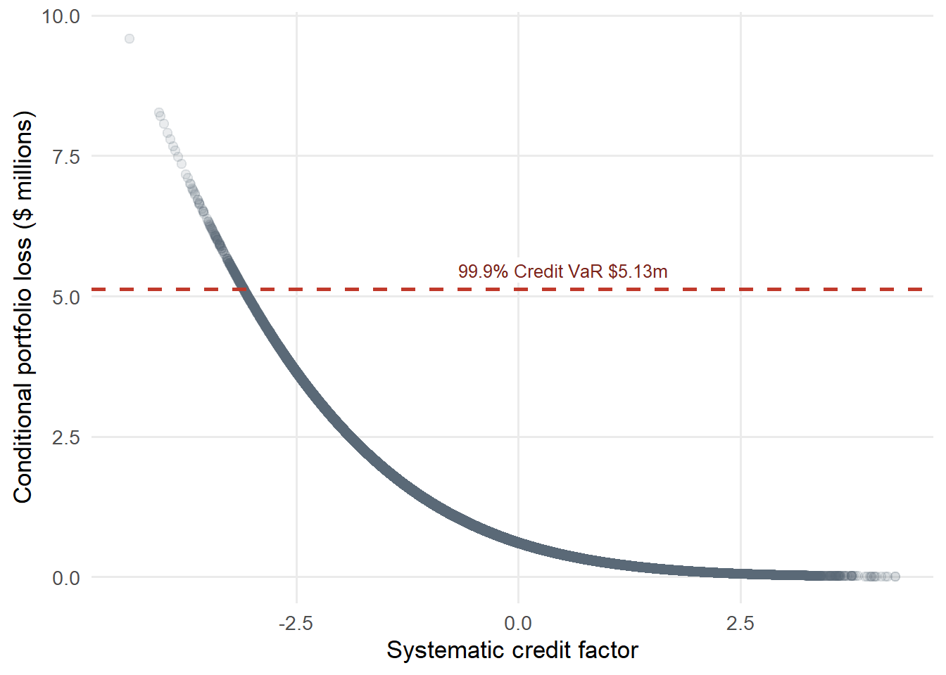
At the 99.9% confidence level, the tail default rate is 12.82%. With $100 million of exposure and 40% LGD, the Credit VaR is $5.13m. Expected loss is much smaller at $0.80m. The difference, $4.33m, is an estimate of economic capital.

Code

kable(
  credit_var_999_table,
  caption = "The 99.9% Gaussian Credit VaR calculation.",
  row.names = FALSE,
  escape = FALSE
)

The 99.9% Gaussian Credit VaR calculation.
Quantity	Value
Tail default rate at 99.9%	12.82%
Credit VaR at 99.9%	$5.13m
Expected loss	$0.80m
Economic capital at 99.9%	$4.33m
Expected shortfall at 99.9%	$5.78m

Expected shortfall adds one more tail-risk measure. Credit VaR identifies a high percentile of losses. Expected shortfall averages the simulated losses that exceed that percentile. The number is larger than VaR because it looks inside the tail after the VaR threshold has been crossed.

The simulation below uses the one-factor representation behind the approximation. A low value of the systematic factor represents a bad economy. Those bad common-factor states raise the conditional default rate and therefore raise portfolio loss.

Code

vasicek_factor_plot_data <- data.frame(
  Systematic_factor = systematic_factor,
  Loss = vasicek_loss / 1e6
)

ggplot(vasicek_factor_plot_data, aes(x = Systematic_factor, y = Loss)) +
  geom_point(size = 2.15, alpha = 0.12, color = "#566573") +
  geom_hline(yintercept = credit_var_loss[3] / 1e6, color = "#C0392B", linetype = "dashed", linewidth = 1) +
  annotate(
    "label",
    x = quantile(systematic_factor, 0.96),
    y = credit_var_loss[3] / 1e6,
    label = paste0("99.9% Credit VaR ", fmt_musd(credit_var_loss[3])),
    hjust = 1,
    vjust = -0.25,
    size = 3.4,
    fill = "white",
    label.size = 0,
    linewidth = 0,
    color = "#7B241C"
  ) +
  labs(
    x = "Systematic credit factor",
    y = "Conditional portfolio loss ($ millions)"
  ) +
  theme_minimal(base_size = 13) +
  theme(panel.grid.minor = element_blank())

Figure 5.11: Systematic factor and conditional portfolio loss.

The t-copula comparison turns this into a model-risk question. The Gaussian Vasicek formula is the analytical benchmark. The Gaussian simulation checks the same logic with a granular portfolio of 1,000 equal loans. The t-copula simulations keep the same one-year PD, total exposure, recovery, and correlation parameter, then change the tail shape of the credit-state scores.

Code

kable(
  credit_model_risk_table,
  caption = "Credit VaR model risk under Gaussian and t-copula assumptions.",
  row.names = FALSE,
  escape = FALSE
)

Credit VaR model risk under Gaussian and t-copula assumptions.
Model	df	EL	VaR 99%	VaR 99.9%	ES 99.9%	Capital 99.9%
Vasicek formula	-	$0.80m	$3.29m	$5.13m	$5.78m	$4.33m
Gaussian sim	-	$0.80m	$3.32m	$5.16m	$5.89m	$4.36m
t-copula sim	10	$0.80m	$6.32m	$11.40m	$13.49m	$10.60m
t-copula sim	4	$0.81m	$9.88m	$17.40m	$19.81m	$16.59m

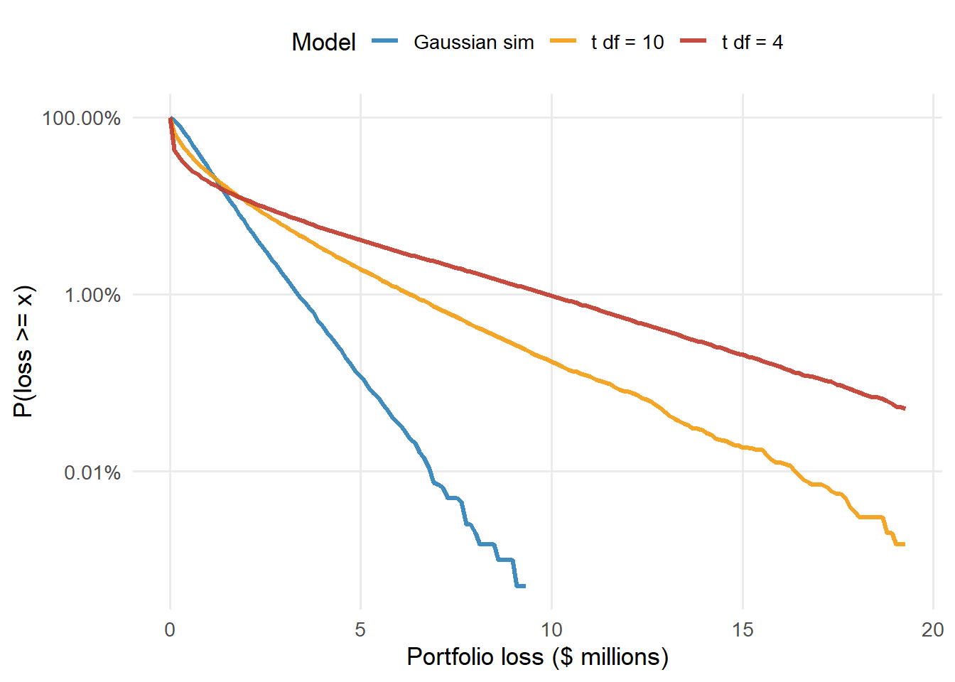
The expected loss rows stay near $0.80m because every model uses the same average one-year PD, EAD, and LGD. The capital rows respond to joint tail behavior. In this run, the Gaussian simulation produces 99.9% capital of $4.36m. The t-copula with 4 degrees of freedom produces $16.59m.

Code

credit_tail_plot_data <- data.frame(
  Loss = rep(credit_tail_grid / 1e6, times = ncol(credit_tail_survival)),
  Survival = as.vector(credit_tail_survival),
  Model = factor(
    rep(colnames(credit_tail_survival), each = length(credit_tail_grid)),
    levels = colnames(credit_tail_survival)
  )
)

ggplot(
  subset(credit_tail_plot_data, !is.na(Survival) & Survival > 0),
  aes(x = Loss, y = Survival, color = Model)
) +
  geom_line(linewidth = 1.1, alpha = 0.9) +
  scale_color_manual(values = c("#2C7FB8", "#F39C12", "#C0392B")) +
  scale_y_log10(labels = function(x) fmt_pct(x, 2)) +
  labs(
    x = "Portfolio loss ($ millions)",
    y = "P(loss >= x)",
    color = "Model"
  ) +
  theme_minimal(base_size = 13) +
  theme(
    legend.position = "top",
    panel.grid.minor = element_blank()
  )

Figure 5.12: Loss-tail survival probabilities under Gaussian and t-copulas.

The chapter’s main gain is a portfolio view of credit risk. PDs describe average default risk name by name. The copula supplies the co-default mechanism. Exposures and recoveries translate default scenarios into dollar losses. Credit VaR, expected shortfall, and economic capital summarize the tail of the resulting loss distribution.

The final comparison turns the copula choice into a capital question. A Gaussian copula and a t-copula can use the same PD, exposure, recovery, and correlation inputs while producing different tail losses. The model choice is therefore a capital assumption as well as a dependence assumption. That is the practical bridge from Hull’s copula example to credit portfolio management: the useful question is how large the portfolio loss can become when defaults arrive together.