The previous chapter used Merton to turn equity, debt, volatility, and the risk-free rate into a model-implied probability of default. That was a structural route to credit risk. In practical terms, it was a capital-structure perspective. Default occurred when the firm’s asset value fell below the promised debt payment. This chapter changes the object being priced. It asks how default risk appears in the prices of corporate bonds and in credit default swap spreads.
The financial question is practical:
Given a corporate bond spread, a recovery assumption, and a default model, is the bond paying enough compensation for credit risk?
This question is practical for a credit analyst, a fixed-income investor, a bank treasury desk, and a risk manager. A corporate bond pays coupons and also exposes the investor to the issuer’s default risk. A credit spread is the extra yield over a default-free benchmark that investors demand for bearing that risk. A credit default swap, or CDS, prices a related contract. The protection buyer pays a periodic premium, and the protection seller pays if the reference entity defaults.
Most of the chapter stays in discrete time. That choice is deliberate. We will use yearly periods so that survival probabilities, marginal default probabilities, recovery payments, bond cash flows, and CDS cash flows can be read directly from tables. When we replicate Hull’s CDS valuation example, we keep the annual payment grid but use Hull’s continuous hazard-rate and discounting conventions. That small change lets us match the book’s CDS numbers while preserving the same table-by-table valuation logic.
The route through the chapter is sequential. First, we build the default timeline with survival probabilities. Second, we price a risky zero-coupon bond. Third, we extend the same logic to a coupon bond. Fourth, we separate real-world and risk-neutral default probabilities. Fifth, we value a simple CDS, connect the CDS fair spread to the Merton PD from the previous chapter, and use Hull’s accrued-premium example as a benchmark for sensitivity and mark-to-market analysis. Finally, we use a real Ford Motor Credit bond as a frozen market-data example to ask whether the observed spread is high or low relative to a simple default model.
Every section repeats the same valuation discipline. First identify the promised cash flows. Then decide which states produce those cash flows. Then attach survival and default probabilities to those states. Finally discount the probability-weighted cash flows and compare the model value with the market quote. This order is necessary because a credit spread by itself is only a compact market summary of promised payments, default timing, recovery, discounting, and compensation for credit risk.
The market example uses Ford Motor Credit Company LLC 2.900% notes due February 10, 2029. The note terms are taken from the SEC free writing prospectus for that issue (Ford Motor Credit Company LLC 2022). The market inputs are frozen for reproducibility. A clean mid price of 94.085 and a mid yield of 5.279% are taken from BondWatch’s page for ISIN US345397B934 (BondWatch 2026). The risk-free benchmark is the 3-year U.S. Treasury constant maturity yield of 4.09% reported in the Federal Reserve H.15 release for June 1, 2026 (Board of Governors of the Federal Reserve System 2026). These teaching inputs make the example reproducible; a live trading recommendation would require current bid and ask quotes, accrued interest, curve construction, liquidity analysis, and position-level constraints.
Before introducing new notation, keep the output of the previous chapter in view. Merton gave a model-implied debt value and a model-implied credit spread for the Hull firm. Those quantities were the spread and debt value that make the structural model internally consistent.
Merton quantities carried into the credit-spread chapter.
Quantity
Value
Merton risk-neutral PD
12.6971%
Model-implied debt value
9.3954
Promised debt payment
10
Merton-implied debt spread
123.7 bps
Read the table as a bridge between chapters. The Merton risk-neutral PD tells us how much probability weight the structural model puts on default states. The promised debt payment tells us what creditors are owed at maturity. The model-implied debt value and spread show how the same default risk appears in debt pricing.
This chapter changes the object being priced. The Merton chapter valued the firm’s equity as an option on assets. Here we price risky debt and CDS protection directly. The logic remains the same. A default probability becomes useful for valuation only after we specify recovery, discounting, promised cash flows, and the market compensation required for bearing credit risk.
The valuation functions used throughout the chapter are shown below. They are deliberately small. Each function corresponds to one financial object. The objects are discounting, survival/default timing, risky bond pricing, CDS premium and protection legs, and the Hull-style accrued-premium CDS calculation.
Start with one firm and a yearly timeline. Let \(h_t\) denote the conditional probability that the firm defaults during year \(t\), given that it survived to the beginning of that year. In this chapter, \(h_t\) is the discrete default rate for the period.
The conditional wording is important. A year-4 default can happen only for firms that reached the beginning of year 4. For valuation, this means we need two different probability objects. Survival probabilities weight the payments made in non-default states. Marginal default probabilities weight the recovery payments made in default states.
Let \(S_t\) denote the probability that the firm survives through the end of year \(t\). We begin with \(S_0=1\) because the firm is alive at time 0. If the conditional default probability in year \(t\) is \(h_t\), then:
\[
S_t=S_{t-1}(1-h_t).
\]
The marginal probability of default in year \(t\) is:
\[
q_t=S_{t-1}h_t.
\]
This expression is easy to read. The firm must first reach the beginning of year \(t\), which has probability \(S_{t-1}\). Then it defaults during year \(t\), conditional on being alive, with probability \(h_t\).
For example, suppose the conditional default probability is 2.5% per year for five years. Then the default timeline is:
Discrete default timeline with a constant 2.5% conditional PD.
Year
ht
St-1
qt
St
1 - St
1
2.50%
100.00%
2.50%
97.50%
2.50%
2
2.50%
97.50%
2.44%
95.06%
4.94%
3
2.50%
95.06%
2.38%
92.69%
7.31%
4
2.50%
92.69%
2.32%
90.37%
9.63%
5
2.50%
90.37%
2.26%
88.11%
11.89%
Notice that the marginal default probability declines slightly through time even though the conditional default probability is constant. The reason is mechanical. Fewer firms remain alive at the beginning of later years. A 2.5% default rate applied to a smaller surviving population gives a smaller unconditional default probability.
The second row shows the logic numerically. The firm reaches the beginning of year 2 with probability 97.50%. Applying the same conditional PD of 2.50% gives a year-2 marginal default probability of 2.44%. That marginal probability is the weight used for a recovery payment in year 2.
The cumulative default probability by year 5 is 11.89%, which is lower than \(5 \times 2.5\%=12.5\%\). Compounding changes the result because the firm cannot default in year 5 if it already defaulted in an earlier year.
The table carries the important accounting. At each horizon, the survival probability and the cumulative default probability add up to 100%. The firm has either defaulted by that date or survived through that date. The rest of the chapter uses exactly these columns. \(S_t\) is used for promised payments that require survival, and \(q_t\) is used for recovery payments that occur only in default states.
4.2 A risky zero-coupon bond
Start with a zero-coupon bond because it has only one promised payment. This keeps the default mechanics visible. Once the single-payment case is clear, a coupon bond is just the same logic repeated across coupon dates.
A risk-free zero-coupon bond with face value \(F\) and maturity \(T\) pays \(F\) with certainty at maturity. Its price is:
\[
B_0^{rf}=\frac{F}{(1+r)^T}.
\]
A risky zero-coupon corporate bond pays different amounts in different credit states. If the issuer survives to maturity, the investor receives the face value \(F\). If the issuer defaults during year \(t\), the investor receives a recovery payment. In this simple example, recovery is a fixed fraction \(R\) of face value, paid at the end of the default year. The risky price is:
\[
B_0^{risky}
=
\sum_{t=1}^{T}\frac{R F q_t}{(1+r)^t}
+
\frac{F S_T}{(1+r)^T}.
\]
The first term is the present value of expected recovery payments. It uses \(q_t\) because recovery is paid in the year default occurs. The second term is the present value of the promised face value weighted by survival to maturity. It uses \(S_T\) because the full face value is paid only if the issuer reaches maturity.
The code below implements the equation directly. In price_zero_defaultable(), recovery_leg is the summation over default years, and survival_leg is the survival-weighted face value at maturity.
Use \(F=100\), \(r=4\%\), \(R=40\%\), maturity of five years, and the same 2.5% conditional default probability. The risk-free value and risky value are:
The risky bond is worth 76.663, while the risk-free bond is worth 82.193. The difference of 5.530 is the present-value cost of default risk under these assumptions. The spread is the extra yield that summarizes this lower price using the promised face value. In this example, the risky yield is 5.459%, so the spread over the 4% risk-free rate is 145.9 basis points.
This yield is a pricing convention. It is the constant yield that makes the promised face value of 100 match the risky price today. It should be read together with the default assumptions that generated the price.
The approximation many credit analysts remember is:
\[
s \approx h(1-R).
\]
In the example, this gives:
\[
s \approx 0.025(1-0.40)=0.015,
\]
or about 150 basis points. The exact spread from the five-year zero-coupon calculation is 145.9 basis points. The approximation is close because the example uses a flat conditional default probability and a simple recovery assumption.
The approximation is useful as a quick diagnostic. With a 2.5% annual conditional PD and 60% loss given default, the annual expected credit loss is about 1.5% of face value. The full valuation adds discounting, compounding, and the fact that default can occur in different years.
4.3 A risky coupon bond
Most corporate bonds pay coupons. The pricing logic is the same, but now the investor receives coupons only while the issuer survives. Let \(C\) denote the annual coupon payment. In this simplified annual-payment model, coupons are paid at the end of each year only if the issuer survives through that year. If default occurs during year \(t\), the model pays recovery at the end of that year and stops the remaining promised coupons and principal. The risky coupon bond price is:
The expected coupon payments while the firm survives.
The expected recovery payments if the firm defaults.
The expected principal payment if the firm survives to maturity.
The code mirrors this decomposition. In price_coupon_defaultable(), the objects named coupon_leg, recovery_leg, and principal_leg correspond to the three terms in the equation. This naming is deliberate because it lets us inspect the valuation directly.
Use a 5-year bond with face value 100 and annual coupon rate 5%. Keep \(r=4\%\), \(R=40\%\), and the 2.5% conditional default probability. The risk-free coupon bond price and risky coupon bond price are:
The risky coupon bond is worth 97.348. Its risk-free counterpart is worth 104.452. The price difference of 7.104 comes from the three probability-weighted cash-flow pieces in the pricing equation. The next table decomposes the risky price.
Read the table from top to bottom. The coupon leg is the present value of coupons paid in survival states. The recovery leg appears in default states. The principal leg is the promised principal weighted by survival to maturity. Adding these three pieces gives the risky bond price.
In this example, survival-weighted coupons contribute 20.685, expected recovery contributes 4.243, and survival-weighted principal contributes 72.420. The principal leg is still the largest component because most of the promised value is concentrated at maturity.
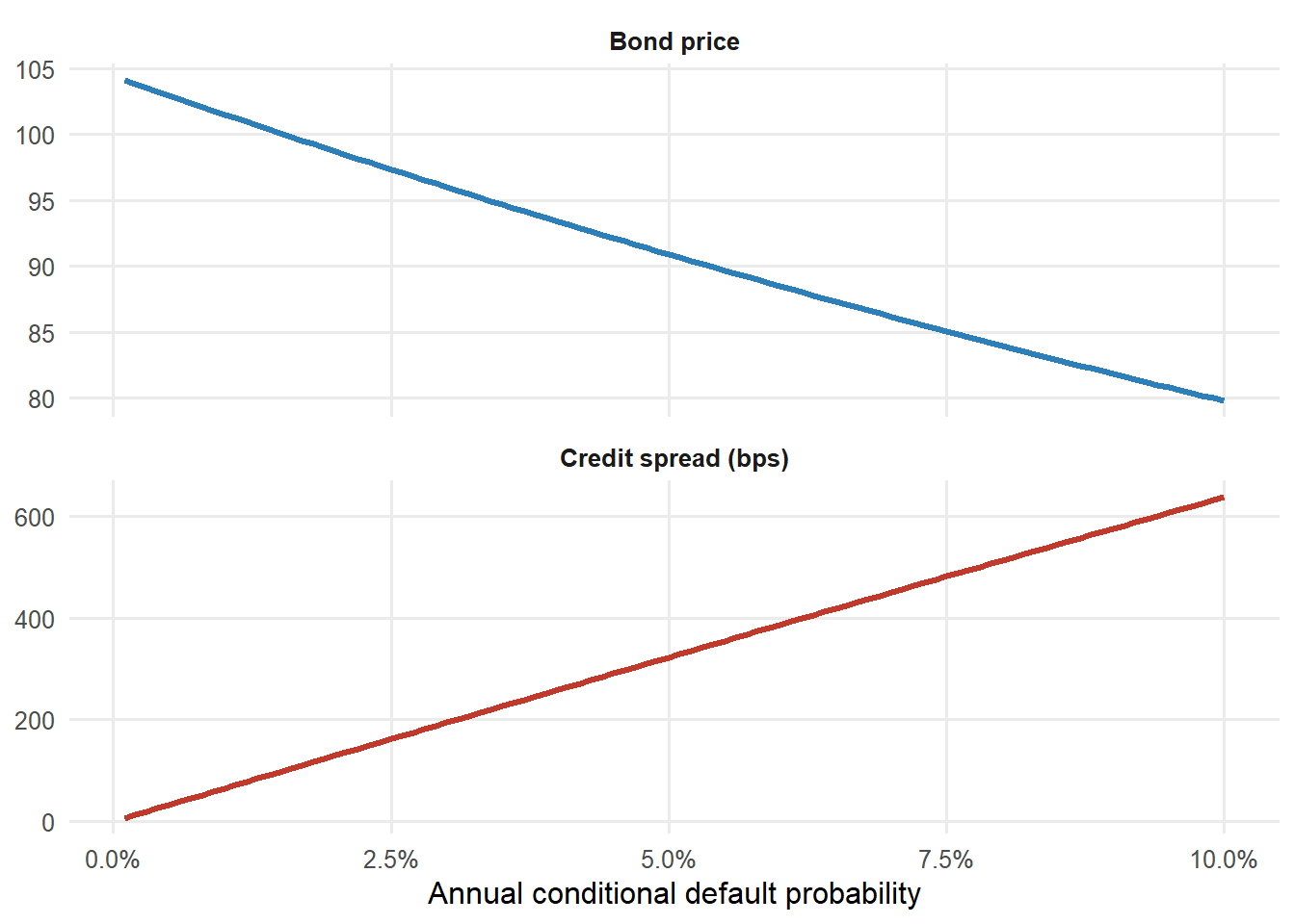
The figure below varies the conditional default probability and reprices the coupon bond. This is the valuation mechanics behind the phrase “credit spreads widen.” Higher default risk lowers the bond price and raises the yield spread.
Figure 4.1: Coupon bond price and yield spread as conditional default risk changes.
The economic interpretation is direct. As default risk rises, investors pay less today for the same promised coupon and principal. Since the promised cash flows stay the same, the lower price mechanically means a higher yield and a higher credit spread. The two panels are therefore the same credit-risk story in two units. Price units appear on the left, and yield-spread units appear on the right.
At this point, the bond-pricing block has established the following map.
Code
credit_spread_bond_checkpoint <-data.frame(Object =c("Conditional PD","Survival probability","Marginal default probability","Recovery","Risky bond price","Credit spread" ),`What it does`=c("Sets the default intensity for each period.","Weights promised coupons and principal.","Weights recovery payments in default years.","Determines loss severity if default occurs.","Discounts probability-weighted promised and default cash flows.","Summarizes the lower risky price as extra yield over the risk-free benchmark." ),`Where it appears in code`=c("`h`","`survival_end` or `S_t`","`marginal_pd` or `q_t`","`recovery`","`price_zero_defaultable()` and `price_coupon_defaultable()`","`coupon_bond_ytm(price) - r`" ),check.names =FALSE)kable( credit_spread_bond_checkpoint,caption ="Checkpoint after the risky bond valuation block.",escape =FALSE,row.names =FALSE)
Checkpoint after the risky bond valuation block.
Object
What it does
Where it appears in code
Conditional PD
Sets the default intensity for each period.
h
Survival probability
Weights promised coupons and principal.
survival_end or S_t
Marginal default probability
Weights recovery payments in default years.
marginal_pd or q_t
Recovery
Determines loss severity if default occurs.
recovery
Risky bond price
Discounts probability-weighted promised and default cash flows.
price_zero_defaultable() and price_coupon_defaultable()
Credit spread
Summarizes the lower risky price as extra yield over the risk-free benchmark.
coupon_bond_ytm(price) - r
4.4 Real-world PDs and risk-neutral PDs
At this point it is tempting to say that the bond spread tells us “the probability of default.” That wording is too quick. A bond spread is a market price. A default probability used to price the bond is therefore a pricing probability. In the notation used earlier in the book, it is closer to a risk-neutral or market-implied probability than to a historical default frequency.
This distinction connects directly with the previous chapters. A credit-scoring model estimates how frequently borrowers with certain characteristics default. A Merton model gives a risk-neutral default weight under an option-pricing structure. A bond spread reflects what the market requires to hold a risky cash-flow claim. These objects can inform each other, but they answer different questions.
What default risk is consistent with market prices?
Risk-neutral or market-implied PD
bond pricing, CDS pricing, relative value, hedging
The numerical difference can be large even in a simple one-year approximation. Suppose an analyst estimates a real-world one-year PD of 1.00% and assumes 40% recovery. The default-loss-only spread approximation is:
\[
s_{\mathrm{loss}} \approx h(1-R).
\]
If the observed market spread is 120 basis points, the spread-implied default rate under the same recovery assumption is higher:
Historical PDs and spread-implied PDs answer different questions.
Quantity
Value
Real-world PD assumption
1.00%
Recovery assumption
40%
Default-loss-only spread
60.0 bps
Observed market spread
120.0 bps
Extra spread over default-loss-only amount
60.0 bps
Spread-implied h from market spread
2.00%
The real-world expected default loss in this example corresponds to only 60.0 basis points. The market spread is 120.0 basis points. Reading the whole spread as default compensation would imply a conditional default rate of 2.00%, while the historical estimate was only 1.00%. The gap is the reason we treat spread-implied probabilities as pricing inputs, separate from direct historical forecasts.
A real-world PD can be lower than a market-implied PD because investors require compensation for bearing systematic credit risk, illiquidity, tax effects, and uncertainty about recovery. A spread-implied default probability therefore needs adjustment before it is interpreted as a literal forecast.
For valuation, the practical consequence is simple. If the analyst priced the bond with the 1.00% real-world PD alone, the default-loss spread would be 60.0 basis points. The market spread of 120.0 basis points embeds more compensation than that. The extra compensation may reflect risk premia, liquidity, recovery uncertainty, or model error.
This chapter uses market-implied probabilities for valuation. That is consistent with the Merton chapter. Merton’s \(N(-d_2)\) is a risk-neutral default weight implied by the option-pricing structure of the model. The next section uses that same idea in a CDS example.
4.5 CDS valuation in annual periods
A CDS is a credit insurance contract in swap form. The protection buyer pays a spread, usually quoted in basis points per year, until maturity or default. The protection seller pays if a credit event occurs. Industry descriptions often call these two sides the premium leg and the protection leg (CFA Institute 2026).
CDS valuation is useful here because it isolates default compensation. A corporate bond mixes coupon income, principal repayment, interest-rate exposure, and default risk. A CDS focuses on the cost of buying or selling protection against default for a reference entity.
In this simplified annual model, the protection leg is:
The notional is \(N\). The loss given default is \(1-R\). The marginal default probability in year \(t\) is \(q_t\). The discount factor brings the expected default payment back to today.
The spread \(s\) is the annual CDS premium as a decimal. The term
\[
\sum_{t=1}^{T}\frac{S_t}{(1+r)^t}
\]
is the risky annuity. It is the present value of one unit paid each year while the issuer survives.
The risky annuity is the premium base of the CDS. It is smaller than a risk-free annuity because premium payments stop after default. The denominator captures that second effect. A high default probability raises expected protection payments and also reduces the number of premium payments the seller expects to receive.
At inception, the fair CDS spread sets the two legs equal:
The numerator is discounted expected default loss per unit of notional. The denominator is the discounted survival-weighted premium base. This formula is the discrete version of the protection-leg versus premium-leg logic used in CDS pricing. It has the same probability structure as the risky bond. Default payments use \(q_t\), while payments made only if the issuer remains alive use \(S_t\).
The code uses two functions. cds_fair_spread() computes the fair spread from the formula above. cds_legs() then checks the result by calculating the protection leg and the premium leg separately.
Now connect this to Merton. The previous chapter estimated a one-year Merton risk-neutral default probability. In the Hull example used there, the model-implied PD is 12.6971%. Treat that as a one-year market-implied input, assume 40% recovery, and value a one-year CDS.
Code
merton_cds_recovery <-0.40merton_cds_h <- pd_mertonmerton_cds_spread <-cds_fair_spread(r = rf,recovery = merton_cds_recovery,h = merton_cds_h)merton_cds_legs <-cds_legs(notional =100,r = rf,recovery = merton_cds_recovery,h = merton_cds_h,spread = merton_cds_spread)merton_cds_table <-data.frame(Quantity =c("Merton risk-neutral one-year PD","Recovery assumption","Loss given default","Fair one-year CDS spread","PV protection leg per 100 notional","PV premium leg per 100 notional" ),Value =c(fmt_pct(pd_merton, 4),fmt_pct(merton_cds_recovery, 0),fmt_pct(1- merton_cds_recovery, 0),paste0(fmt_bps(merton_cds_spread, 1), " bps"),fmt_price(merton_cds_legs$protection_leg, 4),fmt_price(merton_cds_legs$premium_leg, 4) ))kable(merton_cds_table, caption ="A one-year CDS spread implied by the Merton PD.")
A one-year CDS spread implied by the Merton PD.
Quantity
Value
Merton risk-neutral one-year PD
12.6971%
Recovery assumption
40%
Loss given default
60%
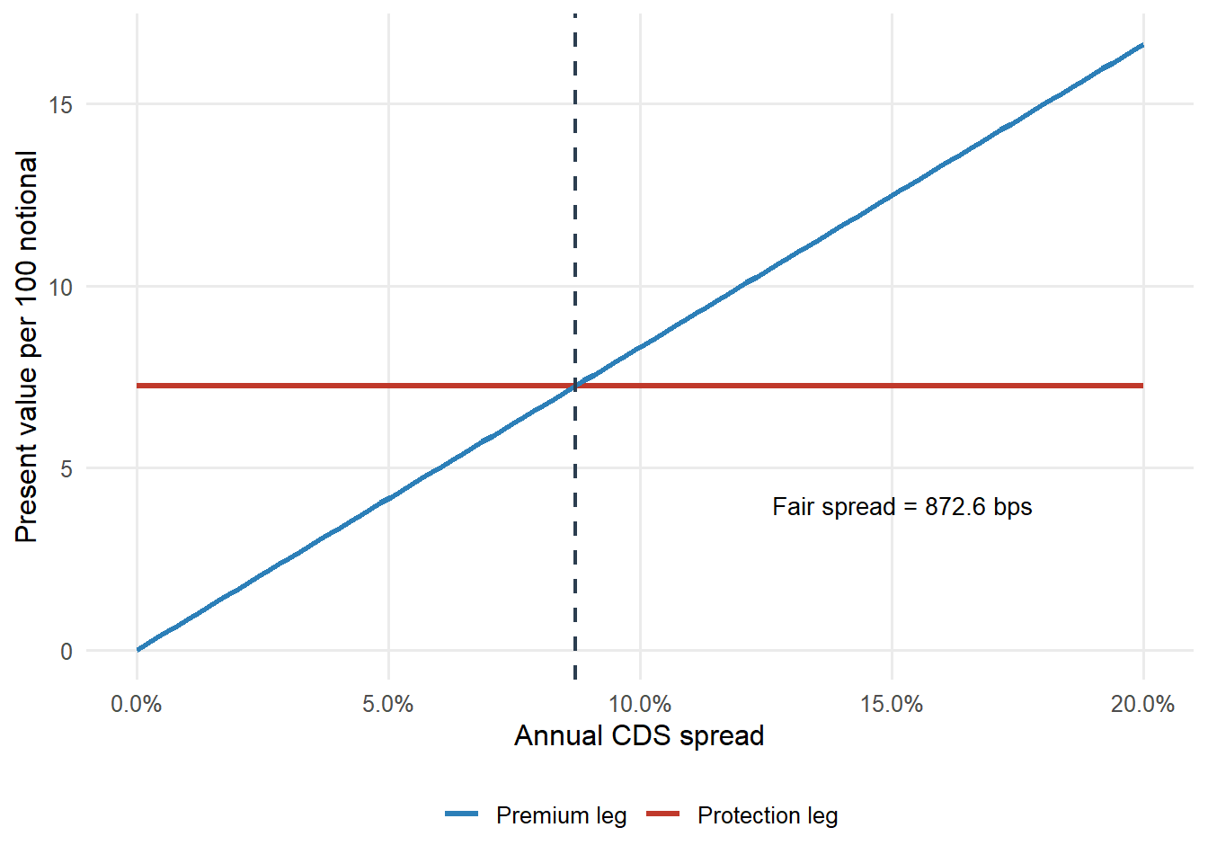
Fair one-year CDS spread
872.6 bps
PV protection leg per 100 notional
7.2555
PV premium leg per 100 notional
7.2555
The fair spread is high because the Merton default probability in this teaching example is high. The spread includes the Merton default probability, the 60% loss given default, and the survival-weighted premium base. At the fair spread, the present value of protection, 7.2555, equals the present value of premiums, 7.2555.
For a one-year CDS, the formula is especially transparent. The fair spread is:
Figure 4.2: CDS premium leg and protection leg as the spread changes.
The red line is flat because the protection leg is fixed once the PD and recovery assumptions are fixed. The blue line rises with the spread because a higher spread means larger premium payments. The fair CDS spread is the crossing point. To the left of the crossing point, the buyer pays too little relative to the modeled protection value. To the right, the buyer pays more than the model requires.
4.6 A Hull-style CDS valuation with accrued premium
The annual CDS formula above is useful because it shows the main economic trade. The protection buyer pays a premium while the issuer survives. The protection seller pays loss given default if the issuer defaults. Section 25.2 of Hull’s book adds two timing details that are important in practice (Hull 2022).
First, default can occur between premium payment dates. For a yearly teaching grid, Hull assumes default occurs halfway through the year in which it happens. Second, if default occurs between premium dates, the protection buyer still owes the premium accrued from the last payment date to the default date. With a midpoint assumption, the accrued premium is one-half of the annual spread for that default year.
The example uses a 5-year CDS, a flat 2.00% hazard rate, a 5.00% continuously compounded risk-free rate, 40% recovery, and notional equal to 1. Let \(a\) denote the flat hazard rate. The survival probability to time \(t\) is:
\[
S(t)=e^{-at}.
\]
The probability of default during year \(t\) is the probability of surviving to the start of that year minus the probability of surviving to the end of that year:
\[
q_t=S(t-1)-S(t).
\]
The following code sets up the Hull-style inputs and creates the survival and default schedule.
Code
hull_hazard <-0.02hull_r <-0.05hull_recovery <-0.40hull_maturity <-5hull_notional <-1hull_components <-hull_cds_components(hazard_rate = hull_hazard,r = hull_r,recovery = hull_recovery,maturity = hull_maturity,notional = hull_notional)hull_schedule <- hull_components$schedulehull_default_table <-data.frame(Year = hull_schedule$year,Survival_to_year_end =fmt_num(hull_schedule$survival_probability, 4),Default_during_year =fmt_num(hull_schedule$default_probability, 4))names(hull_default_table) <-c("Year", "Survival to year end", "Default during year")kable( hull_default_table,caption ="Hull-style survival and default probabilities for a 2% hazard rate.")
Hull-style survival and default probabilities for a 2% hazard rate.
Year
Survival to year end
Default during year
1
0.9802
0.0198
2
0.9608
0.0194
3
0.9418
0.0190
4
0.9231
0.0186
5
0.9048
0.0183
Read one row slowly. At the start of year 3, the issuer has survived two years, so \(S(2)=e^{-0.02\times 2}\), which equals 0.9608. At the end of year 3, \(S(3)=e^{-0.02\times 3}\), which equals 0.9418. The difference, 0.0190, is the unconditional probability of default during year 3.
Now value the regular premium payments. If the annual CDS spread is \(s\), a surviving contract pays \(s\) at each year end. The present value of one expected premium payment is:
\[
s \times S(t) \times e^{-rt}.
\]
The table keeps the unknown spread \(s\) outside the numeric value. This lets us compute the risky annuity first and solve for the fair spread later.
Code
hull_premium_table <-data.frame(Time_years = hull_schedule$year,Survival_probability =fmt_num(hull_schedule$survival_probability, 4),Discount_factor =fmt_num(hull_schedule$premium_discount, 4),PV_of_expected_payment =paste0(fmt_num(hull_schedule$premium_annuity_piece, 4), " x s"))names(hull_premium_table) <-c("Time (years)","Survival probability","Discount factor","PV of expected payment")kable( hull_premium_table,caption ="Present value of expected CDS premium payments in the Hull-style example.")
Present value of expected CDS premium payments in the Hull-style example.
Time (years)
Survival probability
Discount factor
PV of expected payment
1
0.9802
0.9512
0.9324 x s
2
0.9608
0.9048
0.8694 x s
3
0.9418
0.8607
0.8106 x s
4
0.9231
0.8187
0.7558 x s
5
0.9048
0.7788
0.7047 x s
Adding the last column gives a regular premium annuity of 4.0728. Therefore, the present value of regular premium payments is 4.0728 times the annual spread \(s\).
Read year 3 as a concrete example. The survival probability to the end of year 3 is 0.9418, and the discount factor is 0.8607. Multiplying them gives 0.8106. Since the spread \(s\) is still unknown at this point, the year-3 expected premium contribution is \(0.8106 \times s\). The table is therefore building the risky annuity one year at a time.
The protection leg is paid if default occurs. With 40% recovery, the loss given default is 60% of notional. Hull’s midpoint convention discounts each expected protection payment from the middle of the corresponding year:
\[
(1-R) \times q_t \times e^{-r(t-0.5)}.
\]
Code
hull_protection_table <-data.frame(Time_years =fmt_num(hull_schedule$default_time, 1),Default_probability =fmt_num(hull_schedule$default_probability, 4),Recovery_rate =fmt_pct(hull_recovery, 0),Expected_payoff =fmt_num(hull_schedule$default_probability * (1- hull_recovery), 4),Discount_factor =fmt_num(hull_schedule$default_discount, 4),PV_of_expected_payoff =fmt_num(hull_schedule$protection_piece, 4))names(hull_protection_table) <-c("Time (years)","Default probability","Recovery","Expected payoff","Discount factor","PV of expected payoff")kable( hull_protection_table,caption ="Present value of expected protection payoff in the Hull-style example.")
Present value of expected protection payoff in the Hull-style example.
Time (years)
Default probability
Recovery
Expected payoff
Discount factor
PV of expected payoff
0.5
0.0198
40%
0.0119
0.9753
0.0116
1.5
0.0194
40%
0.0116
0.9277
0.0108
2.5
0.0190
40%
0.0114
0.8825
0.0101
3.5
0.0186
40%
0.0112
0.8395
0.0094
4.5
0.0183
40%
0.0110
0.7985
0.0088
The sum of the protection column is 0.0506. This is the model value of the default payment per 1 of notional.
The year-3 protection row uses the same discipline with a default payment. The default probability during year 3 is 0.0190. With 40% recovery, the expected payoff before discounting is 0.0114. Discounting from the midpoint of year 3 gives a present value contribution of 0.0101. The protection leg is the sum of those yearly expected default payments.
There is one more premium component. If default occurs halfway through a year, the protection buyer has used half a year of protection since the last payment date. The accrued premium for that default scenario is therefore:
\[
0.5 \times s \times q_t \times e^{-r(t-0.5)}.
\]
Code
hull_accrual_table <-data.frame(Time_years =fmt_num(hull_schedule$default_time, 1),Default_probability =fmt_num(hull_schedule$default_probability, 4),Expected_accrual =paste0(fmt_num(0.5* hull_schedule$default_probability, 4), " x s"),Discount_factor =fmt_num(hull_schedule$default_discount, 4),PV_of_expected_accrual =paste0(fmt_num(hull_schedule$accrual_annuity_piece, 4), " x s"))names(hull_accrual_table) <-c("Time (years)","Default probability","Expected accrued premium","Discount factor","PV of expected accrued premium")kable( hull_accrual_table,caption ="Present value of expected accrued premium in the Hull-style example.")
Present value of expected accrued premium in the Hull-style example.
Time (years)
Default probability
Expected accrued premium
Discount factor
PV of expected accrued premium
0.5
0.0198
0.0099 x s
0.9753
0.0097 x s
1.5
0.0194
0.0097 x s
0.9277
0.0090 x s
2.5
0.0190
0.0095 x s
0.8825
0.0084 x s
3.5
0.0186
0.0093 x s
0.8395
0.0078 x s
4.5
0.0183
0.0091 x s
0.7985
0.0073 x s
The accrued-premium annuity is 0.0422. The total premium base is therefore the regular premium annuity plus the accrued-premium annuity.
Code
hull_summary <-data.frame(Quantity =c("PV regular premium annuity","PV accrued premium annuity","Total risky annuity","PV protection leg","Fair CDS spread" ),Value =c(paste0(fmt_num(hull_components$premium_annuity, 4), " x s"),paste0(fmt_num(hull_components$accrual_annuity, 4), " x s"),paste0(fmt_num(hull_components$risky_annuity_with_accrual, 4), " x s"),fmt_num(hull_components$protection_leg, 4),paste0(fmt_bps(hull_components$fair_spread, 1), " bps") ))kable( hull_summary,caption ="Hull-style fair CDS spread from premium, accrual, and protection legs.")
Hull-style fair CDS spread from premium, accrual, and protection legs.
Quantity
Value
PV regular premium annuity
4.0728 x s
PV accrued premium annuity
0.0422 x s
Total risky annuity
4.1150 x s
PV protection leg
0.0506
Fair CDS spread
123.0 bps
At inception, the fair spread makes the value of the two sides equal:
Solving for \(s\) gives 1.2300%, or 123.0 basis points. This reproduces the key numerical result in Hull’s CDS valuation example while keeping each cash-flow component visible.
The same decomposition also explains mark-to-market value. Suppose an existing 5-year CDS contract was written at 150 basis points, while the current model inputs imply a fair spread of 123.0 basis points. The protection seller is receiving more premium than a new fair contract would require under these inputs, so the existing contract has positive value to the seller.
Code
hull_contract_spread <-0.015hull_mtm_seller <- hull_components$risky_annuity_with_accrual * hull_contract_spread - hull_components$protection_leghull_mtm_buyer <--hull_mtm_sellerhull_mtm_table <-data.frame(Quantity =c("Contractual spread","Current fair spread","PV contractual premium leg","PV protection leg","Value to protection seller","Value to protection buyer" ),Value =c(paste0(fmt_bps(hull_contract_spread, 1), " bps"),paste0(fmt_bps(hull_components$fair_spread, 1), " bps"),fmt_num(hull_components$risky_annuity_with_accrual * hull_contract_spread, 4),fmt_num(hull_components$protection_leg, 4),fmt_num(hull_mtm_seller, 4),fmt_num(hull_mtm_buyer, 4) ))kable( hull_mtm_table,caption ="Mark-to-market value of an existing CDS in the Hull-style example.")
Mark-to-market value of an existing CDS in the Hull-style example.
Quantity
Value
Contractual spread
150.0 bps
Current fair spread
123.0 bps
PV contractual premium leg
0.0617
PV protection leg
0.0506
Value to protection seller
0.0111
Value to protection buyer
-0.0111
The value to the protection seller is 0.0111 per 1 of notional. The value to the protection buyer is the same number with the opposite sign. A CDS is a zero-value contract only when it is initiated at the current fair spread. After the market spread or default assumptions move, an old spread becomes valuable to one side and costly to the other.
Hull also uses the CDS spread in the reverse direction. If the observed 5-year CDS spread is 100 basis points, and we keep the same risk-free rate and recovery assumption, we can solve for the flat hazard rate that makes the CDS fair spread equal to the observed quote.
Implied hazard rate from a CDS spread in the Hull-style example.
Quantity
Value
Observed CDS spread
100.0 bps
Implied flat hazard rate
1.626%
Repriced fair spread at implied hazard
100.0 bps
This is the CDS version of the spread-implied default probability idea. The market spread is observed. Recovery, maturity, and discounting are modeling choices. The hazard rate is the value that makes the premium leg and protection leg balance.
There is a useful recovery lesson here. In a plain-vanilla CDS, the same recovery assumption affects both sides of the calculation when the hazard rate is implied from the CDS spread. A lower recovery raises loss given default, but it also lowers the hazard rate needed to reproduce a given spread. These two effects partially offset each other. In this chapter, recovery remains important because we also use it to interpret risky bond prices and relative-value signals, where the bond’s coupons, principal, and recovery timing all matter.
Replicating Hull is the starting point. The added value for this chapter is to turn that replication into a diagnostic tool. Once the premium annuity, accrued premium, protection leg, and fair spread are explicit, we can ask four practical questions. How close is the quick approximation, how sensitive is the spread to default and recovery assumptions, how valuable is an old contract when its contractual spread differs from the current fair spread, and how much value moves for a one-basis-point spread change?
A first benchmark is the quick approximation:
\[
s \approx a(1-R).
\]
This approximation says that the annual CDS spread should be close to the hazard rate times loss given default. It is useful because it gives the analyst a fast mental check. With Hull’s inputs, the approximation is:
\[
s \approx 0.02(1-0.40)=0.0120.
\]
That is 120 basis points. The full Hull-style valuation gives 123.0 basis points. The difference is small, but it is meaningful because the full valuation includes survival weighting, discounting, midpoint default timing, and accrued premium.
Code
hull_quick_spread <- hull_hazard * (1- hull_recovery)hull_no_accrual_spread <- hull_components$protection_leg / hull_components$premium_annuityhull_approx_table <-data.frame(Method =c("Quick approximation","Hull timing without accrued premium","Hull timing with accrued premium" ),Calculation =c("hazard x LGD","protection leg / regular premium annuity","protection leg / total risky annuity" ),Fair_spread =c(paste0(fmt_bps(hull_quick_spread, 1), " bps"),paste0(fmt_bps(hull_no_accrual_spread, 1), " bps"),paste0(fmt_bps(hull_components$fair_spread, 1), " bps") ),Difference_from_Hull_full =c(paste0(fmt_bps(hull_quick_spread - hull_components$fair_spread, 1), " bps"),paste0(fmt_bps(hull_no_accrual_spread - hull_components$fair_spread, 1), " bps"),"0.0 bps" ))names(hull_approx_table) <-c("Method","Calculation","Fair spread","Difference from full Hull")kable( hull_approx_table,caption ="Quick CDS spread approximation compared with the Hull-style valuation.")
Quick CDS spread approximation compared with the Hull-style valuation.
Method
Calculation
Fair spread
Difference from full Hull
Quick approximation
hazard x LGD
120.0 bps
-3.0 bps
Hull timing without accrued premium
protection leg / regular premium annuity
124.3 bps
1.3 bps
Hull timing with accrued premium
protection leg / total risky annuity
123.0 bps
0.0 bps
The quick approximation is deliberately simple. It treats the spread as expected annual loss. The full Hull-style spread is slightly higher than the quick approximation because the valuation tracks the exact timing of expected premium and protection payments. The version without accrued premium is slightly higher than the full version because it leaves out a payment that benefits the protection seller when default occurs between payment dates. Adding accrued premium increases the premium base, so the fair spread required to balance the protection leg falls.
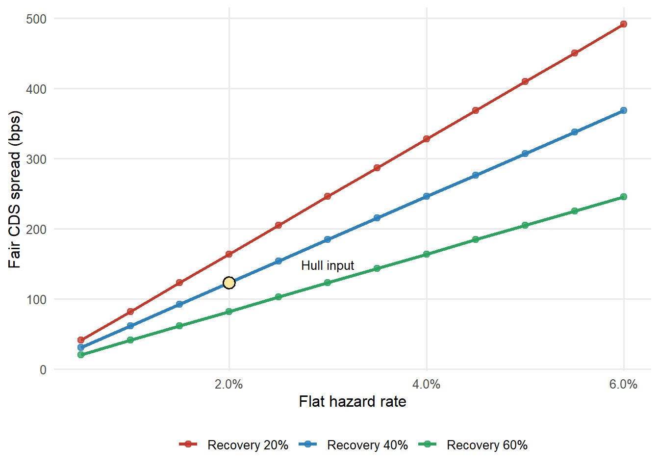
The next graph turns the same machinery into a sensitivity analysis. Keep the 5-year maturity and 5.00% risk-free rate fixed. Change only the flat hazard rate and recovery assumption. Each point reprices the CDS with the same Hull-style functions used above.
Figure 4.3: Fair CDS spread under hazard and recovery assumptions.
The graph gives a useful reading rule. Moving to the right raises the probability of default and therefore raises the protection leg. Moving from low recovery to high recovery lowers loss given default and therefore lowers the spread. The Hull input sits on the 40% recovery line at a 2.00% hazard rate, producing a fair spread of 123.0 basis points.
The sensitivity is also a warning about interpretation. A CDS spread by itself does not reveal a unique default probability unless recovery and maturity are specified. A 120-basis-point spread can be consistent with different hazard rates under different recovery assumptions.
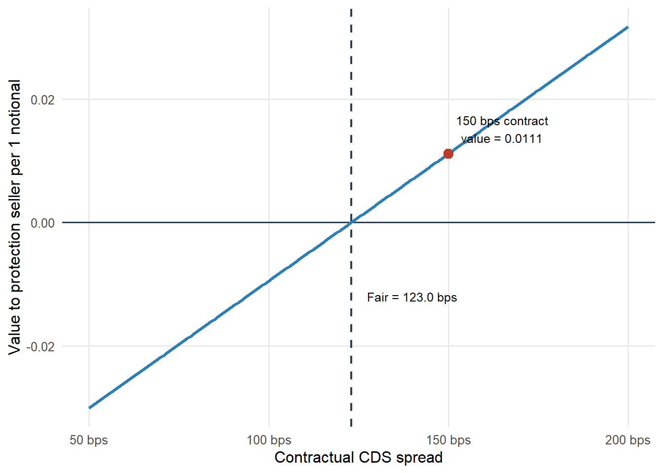
Now use the Hull fair spread as a mark-to-market benchmark. The existing contract in the example pays 150 basis points. The value to the protection seller is:
Figure 4.4: Mark-to-market value to the protection seller as the contractual spread changes.
The vertical dashed line is the current fair spread. At that spread, the contract has zero value at inception. To the right of the dashed line, the contractual spread is higher than the fair spread, so the protection seller receives excess premium and the position has positive value. To the left, the protection buyer has the favorable contract.
The risky annuity also gives a professional risk measure. A one-basis-point move in the contractual spread changes the value by approximately:
hull_cds01_per_unit <- hull_components$risky_annuity_with_accrual *0.0001hull_cds01_notional <- hull_cds01_per_unit *100000000hull_cds01_table <-data.frame(Quantity =c("Total risky annuity","Value change for 1 bp per 1 notional","Value change for 1 bp on 100 million notional" ),Value =c(fmt_num(hull_components$risky_annuity_with_accrual, 4),fmt_num(hull_cds01_per_unit, 7),paste0("$", format(round(hull_cds01_notional, 0), big.mark =",")) ))kable( hull_cds01_table,caption ="CDS01 implied by the Hull-style risky annuity.")
CDS01 implied by the Hull-style risky annuity.
Quantity
Value
Total risky annuity
4.1150
Value change for 1 bp per 1 notional
0.0004115
Value change for 1 bp on 100 million notional
$41,150
For a 100 million notional CDS, a one-basis-point spread change is worth about $41,150 under these assumptions. The risky annuity is useful beyond the fair-spread calculation because it converts spread movements into money.
The Hull replication is therefore doing more than reproducing a textbook number. It creates a compact CDS toolkit.
Code
cds_toolkit_checkpoint <-data.frame(Tool =c("Fair spread","Implied hazard rate","Approximation check","Sensitivity surface","Mark-to-market value","CDS01" ),`Question answered`=c("What spread makes a new CDS worth zero?","What flat default intensity is implied by an observed spread?","Is the quick hazard x LGD rule close enough for a first read?","How does the fair spread move when hazard and recovery change?","Who benefits when an old contractual spread differs from the current fair spread?","How many dollars move for a one-basis-point spread change?" ),`Credit use`=c("Pricing new protection.","Reading market-implied default risk.","Sanity checking quotes.","Stress testing model assumptions.","Valuing existing positions.","Measuring spread risk." ),check.names =FALSE)kable( cds_toolkit_checkpoint,caption ="Checkpoint after the Hull-style CDS valuation block.",row.names =FALSE)
Checkpoint after the Hull-style CDS valuation block.
Tool
Question answered
Credit use
Fair spread
What spread makes a new CDS worth zero?
Pricing new protection.
Implied hazard rate
What flat default intensity is implied by an observed spread?
Reading market-implied default risk.
Approximation check
Is the quick hazard x LGD rule close enough for a first read?
Sanity checking quotes.
Sensitivity surface
How does the fair spread move when hazard and recovery change?
Stress testing model assumptions.
Mark-to-market value
Who benefits when an old contractual spread differs from the current fair spread?
Valuing existing positions.
CDS01
How many dollars move for a one-basis-point spread change?
Measuring spread risk.
4.7 A real corporate bond snapshot
Now use a real corporate bond as a market application. Ford Motor Credit Company LLC issued 2.900% notes due February 10, 2029. The SEC free writing prospectus gives the issuer, coupon, maturity, and note description (Ford Motor Credit Company LLC 2022). BondWatch reports a clean mid price of 94.085 and a mid yield of 5.279% for ISIN US345397B934 (BondWatch 2026). The Federal Reserve H.15 release reports the 3-year Treasury constant maturity yield as 4.09% for June 1, 2026 (Board of Governors of the Federal Reserve System 2026).
We freeze these values in the code to keep the example reproducible. The goal is to show how a credit analyst can translate a quoted spread into a default-risk assumption and then compare that assumption with a simple valuation model.
All bond prices in this example are quoted per 100 of face value. Yield spreads and CDS spreads are quoted in basis points. When the chapter uses CDS values per 1 of notional, it says so explicitly; when it scales to 100 million notional, the output is shown in dollars. Keeping those units separate avoids confusing a bond price, a spread, and a contract value.
Code
ford_inputs <-data.frame(issuer ="Ford Motor Credit Company LLC",isin ="US345397B934",coupon_rate =0.029,maturity_date ="2029-02-10",clean_mid_price =94.085,mid_yield =0.05279,treasury_3y =0.0409,recovery =0.40,teaching_maturity_years =3)ford_inputs_table <-data.frame(Quantity =c("Issuer","ISIN","Coupon","Maturity date","Clean mid price","Mid yield","3-year Treasury benchmark","Recovery assumption","Discrete teaching maturity" ),Value =c( ford_inputs$issuer, ford_inputs$isin,fmt_pct(ford_inputs$coupon_rate, 3), ford_inputs$maturity_date,fmt_price(ford_inputs$clean_mid_price, 3),fmt_pct(ford_inputs$mid_yield, 3),fmt_pct(ford_inputs$treasury_3y, 2),fmt_pct(ford_inputs$recovery, 0),paste0(ford_inputs$teaching_maturity_years, " annual periods") ))kable(ford_inputs_table, caption ="Frozen inputs for the Ford Motor Credit bond example.")
Frozen inputs for the Ford Motor Credit bond example.
Quantity
Value
Issuer
Ford Motor Credit Company LLC
ISIN
US345397B934
Coupon
2.900%
Maturity date
2029-02-10
Clean mid price
94.085
Mid yield
5.279%
3-year Treasury benchmark
4.09%
Recovery assumption
40%
Discrete teaching maturity
3 annual periods
The input table separates three types of information. The coupon, maturity date, and issuer describe the contract. The clean mid price and mid yield summarize the market quote. The Treasury benchmark, recovery assumption, and teaching maturity are modeling choices used to translate the quote into default-risk terms.
The Ford block should be read as a market-data teaching exercise. It uses real security information and real frozen market inputs, then maps them to a deliberately small annual model. That mapping is useful because the cash-flow, survival, recovery, and spread logic can be seen line by line. It is also a limitation because a desk-level valuation would need more market microstructure and bond-convention detail.
Code
ford_teaching_map <-data.frame(Layer =c("Real market input","Teaching approximation","What the approximation gives us","What a desk would add","How to read the result" ),`In this chapter`=c("Issuer, coupon, maturity date, clean mid price, mid yield, and Treasury benchmark are frozen from public sources.","Cash flows are placed on a 3-year annual grid with one flat conditional default probability and one recovery assumption.","The model can translate a quoted spread into default risk and then reprice the same bond under alternative credit views.","Accrued interest, exact coupon dates, day-count convention, full risk-free curve, bid-ask spread, liquidity, seniority, taxes, and comparable CDS quotes.","A relative-value signal conditional on the assumptions, not a live trading recommendation." ),check.names =FALSE)kable( ford_teaching_map,caption ="How the real Ford quote is mapped into the teaching valuation model.",row.names =FALSE)
How the real Ford quote is mapped into the teaching valuation model.
Layer
In this chapter
Real market input
Issuer, coupon, maturity date, clean mid price, mid yield, and Treasury benchmark are frozen from public sources.
Teaching approximation
Cash flows are placed on a 3-year annual grid with one flat conditional default probability and one recovery assumption.
What the approximation gives us
The model can translate a quoted spread into default risk and then reprice the same bond under alternative credit views.
What a desk would add
Accrued interest, exact coupon dates, day-count convention, full risk-free curve, bid-ask spread, liquidity, seniority, taxes, and comparable CDS quotes.
How to read the result
A relative-value signal conditional on the assumptions, not a live trading recommendation.
The observed yield spread over the 3-year Treasury benchmark is:
ford_market_spread <- ford_inputs$mid_yield - ford_inputs$treasury_3yford_approx_h <- ford_market_spread / (1- ford_inputs$recovery)ford_implied_h <-solve_flat_hazard_from_price(price = ford_inputs$clean_mid_price,face =100,coupon_rate = ford_inputs$coupon_rate,r = ford_inputs$treasury_3y,recovery = ford_inputs$recovery,maturity = ford_inputs$teaching_maturity_years)ford_model_price_at_approx_h <-price_coupon_defaultable(face =100,coupon_rate = ford_inputs$coupon_rate,r = ford_inputs$treasury_3y,recovery = ford_inputs$recovery,h =rep(ford_approx_h, ford_inputs$teaching_maturity_years))ford_model_price_at_implied_h <-price_coupon_defaultable(face =100,coupon_rate = ford_inputs$coupon_rate,r = ford_inputs$treasury_3y,recovery = ford_inputs$recovery,h =rep(ford_implied_h, ford_inputs$teaching_maturity_years))ford_cds_spread_at_implied_h <-cds_fair_spread(r = ford_inputs$treasury_3y,recovery = ford_inputs$recovery,h =rep(ford_implied_h, ford_inputs$teaching_maturity_years))ford_spread_table <-data.frame(Quantity =c("Observed yield spread","Approximate h from s / LGD","Price-implied flat h","Model price at approximate h","Model price at price-implied h","CDS fair spread at price-implied h" ),Value =c(paste0(fmt_bps(ford_market_spread, 1), " bps"),fmt_pct(ford_approx_h, 3),fmt_pct(ford_implied_h, 3),fmt_price(ford_model_price_at_approx_h, 3),fmt_price(ford_model_price_at_implied_h, 3),paste0(fmt_bps(ford_cds_spread_at_implied_h, 1), " bps") ))kable(ford_spread_table, caption ="Market spread and default-risk interpretation for the Ford bond.")
Market spread and default-risk interpretation for the Ford bond.
Quantity
Value
Observed yield spread
118.9 bps
Approximate h from s / LGD
1.982%
Price-implied flat h
1.555%
Model price at approximate h
93.379
Model price at price-implied h
94.084
CDS fair spread at price-implied h
94.8 bps
The observed spread is 118.9 basis points. With 40% recovery, the quick spread approximation implies a conditional default probability of 1.982% per year. Solving the discrete risky-bond pricing equation to match the clean price gives a price-implied conditional default probability of 1.555% per year. These two numbers are close because the bond is short-dated in this teaching approximation.
The table is the main output of this step. The observed spread is the market compensation. The approximate default rate is the quick credit-spread translation. The price-implied default rate is the value of \(h\) that makes the simplified risky-bond model reproduce the observed clean price.
The two model prices also explain why we solve for \(h\) after the rule-of-thumb calculation. At the approximate \(h\), the model price is 93.379. At the price-implied \(h\), the model price is 94.084, which matches the observed clean price by construction. The root-solving step forces the model to respect the actual bond price as well as the spread approximation.
The same calculation can be read as a compact credit-spread workflow. This workflow is the applied value of the section. It turns a quoted bond into a default assumption, then turns that default assumption back into a bond or CDS valuation output.
Code
ford_workflow_table <-data.frame(Step =c("1. Observe the bond quote","2. Choose valuation assumptions","3. Translate spread into default risk","4. Reprice the bond","5. Convert the same view into CDS terms","6. Use the result for relative value" ),Question =c("What compensation is the market offering?","Which recovery and discounting assumptions will we use?","What default rate is roughly consistent with the spread?","Which h reproduces the clean price in the risky-bond model?","What CDS spread would price the same default-and-recovery view?","Is the market spread high or low relative to the analyst's view?" ),Ford_output =c(paste0(fmt_bps(ford_market_spread, 1), " bps observed spread"),paste0(fmt_pct(ford_inputs$recovery, 0), " recovery; ", fmt_pct(ford_inputs$treasury_3y, 2), " Treasury rate"),fmt_pct(ford_approx_h, 3),fmt_pct(ford_implied_h, 3),paste0(fmt_bps(ford_cds_spread_at_implied_h, 1), " bps"),"Compare market spread with model spread" ))names(ford_workflow_table) <-c("Step", "Question", "Ford output")kable(ford_workflow_table, caption ="A compact workflow for reading the Ford bond spread.")
A compact workflow for reading the Ford bond spread.
Step
Question
Ford output
1. Observe the bond quote
What compensation is the market offering?
118.9 bps observed spread
2. Choose valuation assumptions
Which recovery and discounting assumptions will we use?
40% recovery; 4.09% Treasury rate
3. Translate spread into default risk
What default rate is roughly consistent with the spread?
1.982%
4. Reprice the bond
Which h reproduces the clean price in the risky-bond model?
1.555%
5. Convert the same view into CDS terms
What CDS spread would price the same default-and-recovery view?
94.8 bps
6. Use the result for relative value
Is the market spread high or low relative to the analyst’s view?
Compare market spread with model spread
The Merton example, the Hull CDS benchmark, and the Ford bond now sit on the same valuation map. Each one starts from a credit-risk input, combines it with recovery and discounting assumptions, and produces a spread-like compensation number. Treat the comparison below as a scale check. It is not an issuer ranking because the Merton firm is a teaching example, Hull’s CDS is a benchmark contract, and the Ford bond is a market snapshot with a different horizon.
Merton, Hull, and Ford translated into CDS-style compensation.
Source
Default input
Horizon
Recovery
Fair CDS spread
Use
Merton teaching firm
12.6971%
1 annual period
40%
872.6 bps
structural model input
Hull CDS benchmark
2.000% flat hazard
5 years
40%
123.0 bps
pricing benchmark
Ford bond price-implied view
1.555% flat h
3 annual periods
40%
94.8 bps
market-implied view
The Merton teaching firm has a much higher default input, so its fair CDS spread is much higher. The Hull row is the clean benchmark because the hazard rate, recovery, maturity, and discounting assumptions are all controlled. The Ford row shows the market application because the bond price is translated into a default view and then into CDS-style compensation. The useful lesson is the mapping. Default input plus recovery produces a protection spread, and the same mapping can be used for structural models, benchmark contracts, and observed bonds.
4.8 Is the bond cheap or expensive?
The phrase “cheap or expensive” needs a benchmark. A bond with a high yield may be paying fair compensation for high default risk. A credit relative-value decision therefore compares the market compensation with the compensation implied by a specific default-and-recovery view.
Choose a pricing view for default and recovery. In this example, the analyst keeps recovery at 40% and tests three possible annual conditional default probabilities.
Reprice the bond under each view, solve for the model-implied yield, and compute the model-implied spread:
A positive spread gap means that the market offers more spread than the model requires. In price terms, that should correspond to a model fair price above the observed market price. The same comparison can be written as:
Positive spread gap and positive price gap both point to the same conclusion. The bond looks cheap under that default assumption. Negative values point to an expensive bond under that assumption.
Code
relative_value_reading_rule <-data.frame(Condition =c("$s_{mkt}>s_{model}$ and $P_{model}>P_{mkt}$","$s_{mkt}<s_{model}$ and $P_{model}<P_{mkt}$","Gap inside the neutral band" ),Signal =c("Cheap under the analyst's credit view","Expensive under the analyst's credit view","Near fair value in this simplified framework" ),Interpretation =c("The market pays more spread than the model requires, and the model values the bond above its market price.","The market pays less spread than the model requires, and the model values the bond below its market price.","The difference is too small to support a strong conclusion after bid-ask spreads and model uncertainty." ))kable( relative_value_reading_rule,caption ="Reading rule for the Ford relative-value exercise.",escape =FALSE)
Reading rule for the Ford relative-value exercise.
Condition
Signal
Interpretation
\(s_{mkt}>s_{model}\) and \(P_{model}>P_{mkt}\)
Cheap under the analyst’s credit view
The market pays more spread than the model requires, and the model values the bond above its market price.
\(s_{mkt}<s_{model}\) and \(P_{model}<P_{mkt}\)
Expensive under the analyst’s credit view
The market pays less spread than the model requires, and the model values the bond below its market price.
Gap inside the neutral band
Near fair value in this simplified framework
The difference is too small to support a strong conclusion after bid-ask spreads and model uncertainty.
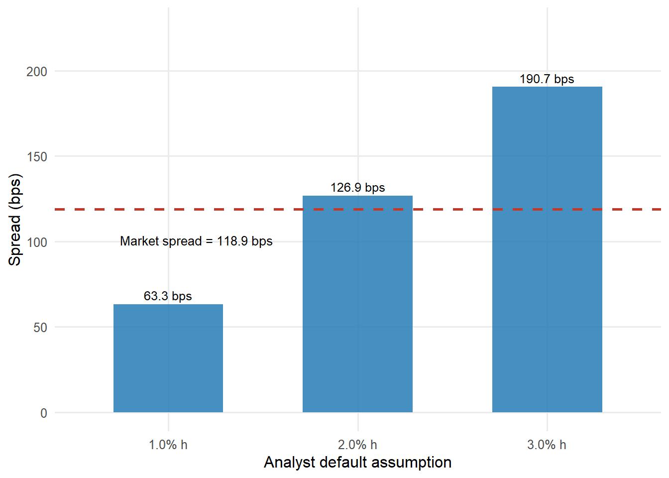
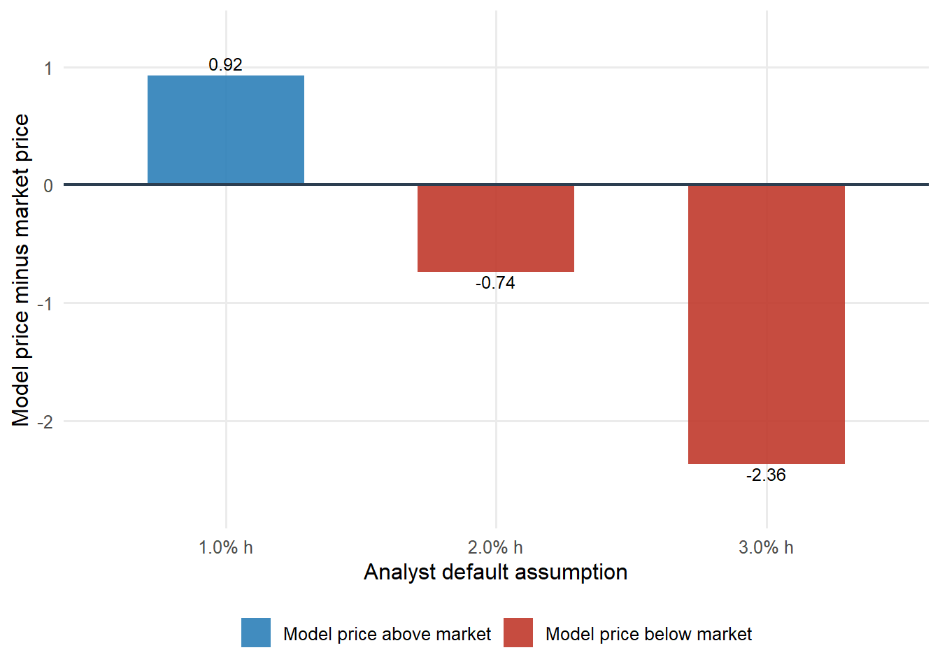
Use the Ford bond as the example. Suppose an analyst believes the fair annual conditional default probability is 1.00%, 2.00%, or 3.00%, with the same 40% recovery and 3-year Treasury benchmark. We also use a 5 basis point neutral band. A spread gap inside that band is treated as near fair value because tiny differences have little economic meaning once bid-ask spreads and model uncertainty are considered. The model-implied price, price gap, spread, and spread gap under each view are:
Relative-value interpretation under alternative default assumptions.
Analyst h
Model price
Model - market price
Model spread
Market - model spread
Signal
1.00%
95.010
0.925
63.3 bps
55.6 bps
Cheap on this view
2.00%
93.349
-0.736
126.9 bps
-8.0 bps
Expensive on this view
3.00%
91.722
-2.363
190.7 bps
-71.8 bps
Expensive on this view
Read the first row carefully. With an annual conditional default probability of 1.00%, the model price is above the market price. The model also says that the fair spread should be below the observed market spread. Those two facts are the same relative-value signal expressed in two units. The market price is low relative to the model price, and the market spread is high relative to the model spread. Under this view, the bond looks cheap.
Now read the last row. With an annual conditional default probability of 3.00%, the model requires more spread than the market offers. The model price falls below the market price. Under this more pessimistic default view, the same bond looks expensive.
The important point is that the trade signal depends on the analyst’s credit view. The market spread is observable. The model spread is conditional on the assumed default probability and recovery rate.
The middle row is useful because it shows the borderline case. At a 2.00% annual conditional default probability, the model spread is 126.9 bps, while the market spread is 118.9 bps. The gap is small enough to read as near fair value in this simplified framework.
This is the practical relative-value workflow. The analyst does not ask whether the bond has a high yield in isolation. The analyst asks whether the observed compensation is high or low relative to a defended credit view. If the default and recovery assumptions are not defensible, the cheap-or-expensive label is not defensible either.
Recovery is part of that credit view. The same market quote can imply a different default rate when recovery changes. A lower recovery means a higher loss given default, so a smaller default probability can explain the same credit compensation. A higher recovery means a lower loss given default, so the same observed spread requires more default risk.
The next table keeps the Ford market price fixed and changes only the recovery assumption. It also shows the relative-value signal if the analyst’s default view is fixed at a 2.00% annual conditional default probability.
Recovery sensitivity for the Ford relative-value signal.
Recovery
Price-implied h
Model spread at h = 2%
Market - model spread
Signal
20%
1.170%
169.3 bps
-50.4 bps
Expensive on this view
40%
1.555%
126.9 bps
-8.0 bps
Expensive on this view
60%
2.319%
85.1 bps
33.8 bps
Cheap on this view
The recovery assumption changes both sides of the interpretation. It changes the default rate implied by the market price, and it changes the model spread required for a fixed analyst default view. This is why recovery deserves the same attention as the PD assumption in credit-spread work.
The direction is worth making explicit. With 20% recovery, the price-implied default rate is 1.170%. With 60% recovery, it rises to 2.319%. The same bond price requires more default probability when the assumed loss per default is smaller.
Figure 4.5: Market spread compared with model-implied spreads under different default assumptions.
The dashed red line is the market spread. The blue bars are model-implied spreads under alternative default assumptions. When the bar is below the red line, the market pays more spread than the model requires. When the bar is above the red line, the market spread is too low for that default view.
Figure 4.6: Model price minus market price under different default assumptions.
Positive bars mean that the analyst’s model values the bond above the market price. That is the price version of a cheap-bond signal. Negative bars mean that the model values the bond below the market price. That is the price version of an expensive-bond signal.
This is a useful relative-value discipline, but it is still a simplified model. The Ford example uses an annual teaching grid, a flat conditional default probability, a single Treasury benchmark, fixed recovery, and clean prices. A trading desk would also check accrued interest, the full risk-free curve, coupon dates, day-count conventions, bid-ask spreads, liquidity, seniority, covenants, taxes, funding costs, ratings migration, and whether a comparable CDS quote exists. These items can make the market spread higher than the default-loss-only spread even when the bond is fairly priced.
The model therefore gives a testable credit view. If the analyst can defend the default probability, recovery rate, and curve inputs, then the spread gap becomes a disciplined measure of compensation. If those inputs are weak, the cheap-or-expensive conclusion is weak as well.
4.9 What this chapter adds
The first chapters estimated default risk from borrower data and firm balance-sheet information. This chapter shows how credit risk is priced in debt markets. A risky bond price is the present value of promised cash flows adjusted for survival, default, and recovery. A CDS spread is the premium that equates the expected discounted protection payment with the expected discounted premium payments.
The chapter can be summarized as an analyst checklist. The checklist is useful because it keeps three objects separate. These are the observed market spread, the model-implied fair spread, and the credit assumptions that connect them.
Code
credit_spread_checklist <-data.frame(Step =c("1. Define the instrument","2. Choose the risk-free benchmark","3. Specify recovery","4. Translate the market spread","5. Reprice the bond or CDS","6. Compare market and model spreads","7. Stress the assumptions" ),Analyst_question =c("What promised cash flows are being priced?","Which default-free curve or benchmark is the comparison point?","How much value is recovered if default occurs?","What default rate is roughly implied by the observed spread?","What spread or price follows from the analyst's default view?","Does the market pay more or less than the model requires?","Does the conclusion survive changes in PD, recovery, and liquidity assumptions?" ),Output =c("coupon, maturity, face value, seniority","discount factors or benchmark yield","recovery rate and loss given default","spread-implied h or PD","model price, fair spread, or fair CDS spread","spread gap and price gap","robust, fragile, or inconclusive signal" ))names(credit_spread_checklist) <-c("Step", "Analyst question", "Output")kable(credit_spread_checklist, caption ="Credit-spread and CDS valuation checklist.")
Credit-spread and CDS valuation checklist.
Step
Analyst question
Output
1. Define the instrument
What promised cash flows are being priced?
coupon, maturity, face value, seniority
2. Choose the risk-free benchmark
Which default-free curve or benchmark is the comparison point?
discount factors or benchmark yield
3. Specify recovery
How much value is recovered if default occurs?
recovery rate and loss given default
4. Translate the market spread
What default rate is roughly implied by the observed spread?
spread-implied h or PD
5. Reprice the bond or CDS
What spread or price follows from the analyst’s default view?
model price, fair spread, or fair CDS spread
6. Compare market and model spreads
Does the market pay more or less than the model requires?
spread gap and price gap
7. Stress the assumptions
Does the conclusion survive changes in PD, recovery, and liquidity assumptions?
robust, fragile, or inconclusive signal
The key ideas are:
survival probabilities turn default timing into cash-flow weights;
recovery affects both bond values and CDS spreads through loss given default;
credit spreads are market prices of default risk and differ from pure historical default frequencies;
Merton PDs can be used as risk-neutral inputs for bond or CDS valuation, provided the horizon and recovery assumptions are explicit;
CDS valuation compares the protection leg with the premium leg, and accrued premium enters the valuation when default occurs between payment dates;
CDS sensitivity analysis turns hazard, recovery, and spread movements into fair spreads, mark-to-market values, and CDS01;
relative value means comparing the market spread with a model-implied spread before judging whether a high-yield bond is attractive.
The next chapter moves from one issuer to a portfolio. Once each borrower has a marginal default probability or a spread-implied credit view, the remaining problem is dependence. How likely are several borrowers to default together?