The previous chapter built a transparent logistic-regression benchmark for credit scoring. This chapter keeps the same credit scoring problem, the same training and test split, and the same evaluation logic, while changing the model class. We now use tree-based models, which learn local decision rules for default risk.
The practical question is the same as before. A bank receives an application, observes borrower and loan information, and needs a probability of default that can be turned into an accept-or-reject decision. The new question is whether a more flexible model can sort applicants into risk groups more effectively than the logistic benchmark, and whether that improvement survives when we look at calibration, bad rates, and economic payoff.
The goal is to understand what a tree-based model is doing, why it can capture patterns that a logistic model may miss, and how to compare it fairly against the logistic benchmark. We begin with a single decision tree, then prepare the numerical matrices required by XGBoost, then move to gradient boosted trees, and finally compare the models using AUC, Brier score, calibration, bad rates, and net payoff.
Current supervisory discussions make this comparison practical. The EBA’s 2023 follow-up report on machine learning for IRB models says that financial institutions use or intend to use machine-learning techniques mainly for PD estimation and risk differentiation, including random forests and gradient boosting for risk-driver selection and scoring (European Banking Authority 2023). The same report emphasizes overfitting, data quality, explainability, and validation. This chapter therefore treats XGBoost as a challenger model that must be compared against the logistic benchmark using AUC, calibration, and economic consequences together.
2.1 The same credit scoring benchmark
This chapter uses the same loan-level data set used in Chapter 1. The outcome is still loan_st, where 1 represents default and 0 represents no default. We also keep the same training and test split. That common test set makes the model comparison meaningful because the models are evaluated on the same out-of-sample observations.
The logistic benchmark is the logi_full model from Chapter 1. It uses age, interest rate, grade, loan amount, income, employment length, home ownership, sex, and region. The tree-based models will use the same information. The same warning from Chapter 1 applies. sex was added for teaching purposes, and protected characteristics or possible proxies require legal, ethical, and fairness review in applied credit decisions. The only thing that changes here is the way the model learns from those variables.
In logistic regression, the model has a clear parametric form. A predictor changes the log-odds of default by a fixed amount, holding the other variables constant. Tree-based models are different. They split the data into regions. For example, a tree might first ask whether the interest rate is above a certain value, then ask whether grade is high or low, and then ask whether income is above a threshold. The prediction is built from a sequence of such rules.
This makes tree-based models attractive for credit scoring because credit risk is often shaped by interactions. A high interest rate may be more concerning for one grade than for another. A loan amount may have a different meaning depending on income. A linear logistic model can include interactions, but the analyst has to specify them. A tree-based model can discover some of these interactions directly from the data.
All models in this chapter produce the same kind of output. For applicant \(i\), each model returns a predicted probability of default, denoted \(\hat p_i\). What changes is the construction of \(\hat p_i\). The logistic model builds it from one coefficient equation. A single tree builds it from the observed default rate in one terminal leaf. XGBoost builds it from many small trees that are added together. Since the output is still a PD, the evaluation tools from Chapter 1 remain valid.
The comparison will use the same evaluation logic developed in Chapter 1:
The table is only a preview. We will return to these metrics after explaining how the tree-based models are built. For now, the important point is that the benchmark is fixed. The same data, same outcome, same test set, and same business interpretation will be used throughout the comparison.
There is also a methodological caveat. For teaching purposes, we keep the comparison compact and use the same test set to illustrate model behavior and business metrics. In a production workflow, tuning choices such as tree depth, learning rate, and number of boosting rounds should be selected with cross-validation or a validation set, leaving a final holdout test set for the last evaluation.
2.2 A single decision tree
A decision tree is the simplest tree-based model. It divides the data by asking a sequence of questions. Each question creates a split. At the end of a sequence of splits, each terminal node contains a group of observations with a default rate. In tree terminology, one terminal node is called a leaf and several terminal nodes are called leaves. The default rate in the leaf becomes the predicted probability of default for applicants who fall into that node.
If a terminal node, or leaf, contains \(n_L\) loans and \(d_L\) of them defaulted, the leaf prediction is:
\[
\hat{p}_L = \frac{d_L}{n_L}.
\]
Any new applicant that reaches that leaf receives the same predicted probability \(\hat{p}_L\). The tree therefore still gives one predicted PD to each applicant in the test set, but those PDs are not usually unique applicant by applicant. Applicants assigned to the same terminal leaf share the same predicted PD. This makes the model easy to inspect because each prediction is tied to a path through the tree.
This is very different from logistic regression. Logistic regression creates one smooth scoring equation. A tree creates local rules. The model may say, in effect, that applicants in this region of the data have a default rate of 3%, while applicants in another region have a default rate of 20%. This rule-based structure is why a single tree is useful pedagogically.
The tradeoff is visible from the formula. A leaf-level PD is simple because it is just a historical default rate inside one group. At the same time, all applicants inside that group receive the same PD. The tree can separate risk only through the leaves it creates.
Code
tree_formula <- loan_st ~ age + int + grade +log(l_amnt) +log(income) + emp_len + home + sex + regionsimple_tree <- rpart::rpart( tree_formula,data = train,method ="class",control = rpart::rpart.control(maxdepth =4,minsplit =100,cp =0.001 ))simple_tree
The printed object describes the tree in text form. Each split sends observations to different branches. The variables that appear near the top are the first questions asked by the model, which means they are especially important for this particular tree.
The numbers at the beginning of the printed lines are internal node identifiers used by rpart. They are not the teaching leaf labels used later in the figure. The root is node 1. The left child of a node receives twice the parent number, and the right child receives twice the parent number plus one. This is why node 15 can split into nodes 30 and 31. Those numbers help rpart store the tree structure, but we will relabel the terminal leaves as Leaf 1 to Leaf 5 to make the diagram easier to read.
The rest of each printed line summarizes the training observations in that node. For a line such as 31) log(l_amnt)>=9.041904 81 26 1 (0.32098765 0.67901235) *, the node contains 81 training applicants. The predicted class is 1, which means default. The number 26 is the classification loss in that node. If the node predicts default, 26 non-default observations would be classified incorrectly. The two values in parentheses are the class proportions, first no default and then default. Therefore, the default rate in this terminal node is 0.67901235, or 67.90%. The asterisk means that the node is terminal. No further split is made below that line.
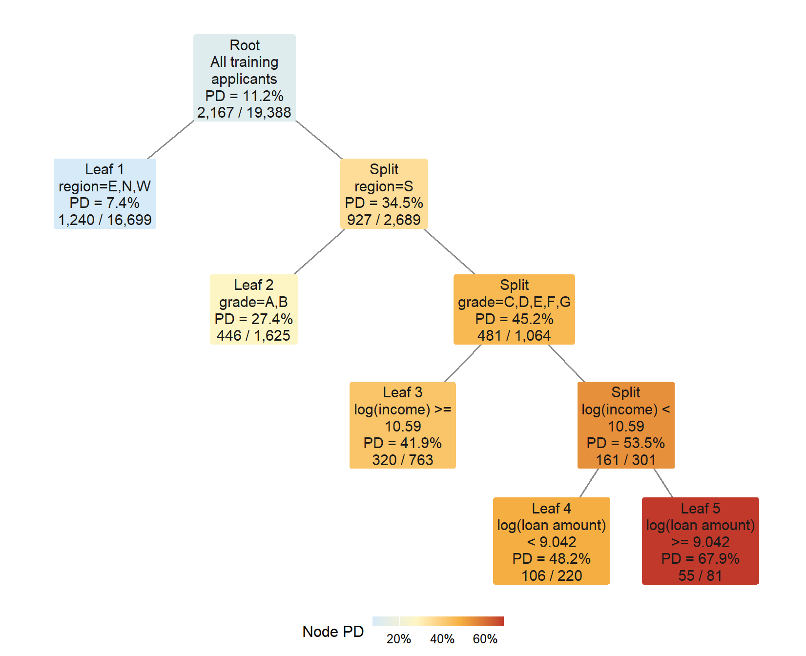
The figure below reads the same fitted tree as a credit-risk map. Each rectangle is one node. To make the diagram easy to read, the terminal boxes are labeled Leaf 1 to Leaf 5 from left to right. Those labels are teaching labels used in the figure and in the table below. The rule printed in a box is the local rule for reaching that box from its parent. The PD is the empirical default rate among applicants in that node. For internal nodes, that rate summarizes the borrowers who have reached that point. For terminal leaves, it becomes the predicted PD assigned to new applicants. The last line shows the same calculation behind the formula above, defaults divided by applicants. Darker colors indicate higher default risk.
Figure 2.1: A single decision tree for credit scoring.
The figure is useful because it makes the scoring logic visible. We will use three words carefully. A split node asks a question and sends applicants to lower nodes. A terminal leaf is where the tree stops and assigns the final predicted PD. A line is one possible answer to a split question. A path is the full route from the root node to one terminal leaf.
In this fitted tree, there are 4 split nodes and 5 terminal leaves. The root is counted as a split node because it creates the first partition of the data. Each box labeled Split is also a split node. None of those split nodes is counted as a leaf. A leaf is counted only when a box has no lines leaving it below. The five terminal boxes are labeled Leaf 1, Leaf 2, Leaf 3, Leaf 4, and Leaf 5 from left to right. A new applicant follows exactly one complete path from the root to one leaf, and the leaf at the end supplies the predicted PD.
The table below expands the same 5 leaves shown in the figure. A terminal box shows its local rule, while the full scoring rule also includes every previous rule on the path. For example, the bottom-right red leaf combines the final loan-amount condition with the previous conditions on region, grade, and income. The table stacks those inherited conditions into one row, so each row is one complete path used for prediction.
The lowest-risk leaf in this fitted tree assigns a PD of 7.43%. The highest-risk leaf assigns a PD of 67.90%. The highest-risk path is Leaf 5, reached by region=S; grade=C,D,E,F,G; log(income) < 10.59; log(loan amount) >= 9.042. This range is the main intuition behind a tree score. Applicants are sorted into different regions of the training data, and each region carries its own historical default rate.
However, a single tree has an important weakness. It can be unstable. A small change in the training data can produce a different set of splits. A tree can also be too simple if it is shallow, or too noisy if it is allowed to grow too deep. This creates a natural motivation for ensemble methods, where many trees are combined to reduce dependence on one tree.
The single tree already produces default probabilities and can be evaluated like the logistic model. In code, simple_tree <- rpart(...) learns the leaves, and predict(simple_tree, newdata = test, type = "prob")[, "1"] returns the leaf default rate assigned to each test applicant. This is the code counterpart of \(\hat p_L = d_L/n_L\). The main role of the single tree in this chapter is conceptual. It shows the basic building block used by more powerful tree-based methods.
The prediction range in the table also shows the limitation of a single tree. The fitted tree has 5 terminal leaves and produces only 5 distinct PD values on the test set. This is useful for explanation because every probability can be traced to a leaf, but it can be too coarse for a scoring system that needs a smoother risk ranking across many applicants.
The next model keeps the leaf idea but changes how leaves are used. Instead of relying on one terminal leaf to supply the whole prediction, XGBoost adds many small trees one after another. Each new tree contributes a correction to a running score. That score is then transformed into a predicted PD.
2.3 Preparing the XGBoost input matrices
Before we slow down the boosting mechanism, we need to build the objects that XGBoost uses. The original credit application data contain both numerical variables and categorical variables. XGBoost requires a numerical matrix, so the first task is to translate the borrower and loan information into one encoded row per applicant.
The translation is handled with model.matrix(). It converts categorical variables such as grade, home, sex, and region into indicator variables, while keeping numerical variables such as age, int, l_amnt, and income in numerical form. This encoding step is important because it makes explicit what the algorithm receives as input. The mathematical object \(x_i\) is represented in code by one row of xgb_train_matrix or xgb_test_matrix; the observed outcome \(y_i\) is represented by xgb_train_label or xgb_test_label.
One row of the matrix is one applicant. Each column is one numerical signal that the algorithm can use when it searches for splits. After this transformation, XGBoost no longer sees a variable called grade as a word or category. It sees numerical columns indicating the applicant’s grade level. This is the bridge between the credit application data and the algorithm.
The translation from the financial object to the R object is:
Code
knitr::kable(data.frame(step =c("Borrower and loan information","Observed default outcome","Encoded numerical matrix","XGBoost score","Predicted probability of default","Credit decision" ),R_object =c("`train` and `test`","`loan_st`","`xgb_train_matrix` and `xgb_test_matrix`","`predict(..., outputmargin = TRUE)` conceptually","`pred_xgb`","cutoff or acceptance-rate rule" ),interpretation =c("Applicant characteristics available before the lending decision","Historical repayment result used for training and evaluation","One row per applicant and one numerical column per model signal","Log-odds scale value produced by the boosted trees","Default-risk estimate after the logistic transformation","Rule that converts the PD into accept or reject" ) ),caption ="Bridge between credit-scoring objects and XGBoost objects.",escape =FALSE)
Bridge between credit-scoring objects and XGBoost objects.
step
R_object
interpretation
Borrower and loan information
train and test
Applicant characteristics available before the lending decision
Observed default outcome
loan_st
Historical repayment result used for training and evaluation
Encoded numerical matrix
xgb_train_matrix and xgb_test_matrix
One row per applicant and one numerical column per model signal
XGBoost score
predict(..., outputmargin = TRUE) conceptually
Log-odds scale value produced by the boosted trees
Predicted probability of default
pred_xgb
Default-risk estimate after the logistic transformation
Credit decision
cutoff or acceptance-rate rule
Rule that converts the PD into accept or reject
The table should be read from top to bottom. The economic object is the loan application, with borrower characteristics and the observed default outcome. The computational object is the encoded matrix, with one row per applicant and one numerical column per signal. XGBoost uses that matrix to build a score on the log-odds scale. The score is converted into a predicted PD, and the PD can then be used by the same cutoff or acceptance-rate rules developed in Chapter 1. This is why the model can be more complex while the credit decision remains familiar.
Code
xgb_formula <-~ age + int + grade +log(l_amnt) +log(income) + emp_len + home + sex + regionxgb_train_matrix <-model.matrix(xgb_formula, data = train)[, -1, drop =FALSE]xgb_test_matrix <-model.matrix(xgb_formula, data = test)[, -1, drop =FALSE]xgb_train_label <-as.numeric(as.character(train$loan_st))xgb_test_label <- actual_default_treexgb_train <- xgboost::xgb.DMatrix(data = xgb_train_matrix,label = xgb_train_label)xgb_test <- xgboost::xgb.DMatrix(data = xgb_test_matrix,label = xgb_test_label)xgb_matrix_dimensions <-data.frame(Object =c("Training matrix", "Test matrix"),Rows =fmt_int(c(nrow(xgb_train_matrix), nrow(xgb_test_matrix))),Columns =fmt_int(c(ncol(xgb_train_matrix), ncol(xgb_test_matrix))))knitr::kable( xgb_matrix_dimensions,caption ="Dimensions of the encoded XGBoost design matrices.",row.names =FALSE)
Dimensions of the encoded XGBoost design matrices.
Object
Rows
Columns
Training matrix
19,388
18
Test matrix
9,695
18
The dimensions table confirms the object that XGBoost will receive. The training matrix is used to learn the boosted trees. The test matrix is held out for the same out-of-sample evaluation used throughout the book. With these objects prepared, we can now inspect how boosting rounds change a prediction before estimating the final model used in the benchmark.
2.4 From trees to boosted trees
XGBoost is easier to understand if we think in terms of a score rather than a final yes/no decision. A single tree gives one set of rules. XGBoost starts from a base score and then adds many small trees as corrections to that score. The corrected score is transformed into a predicted probability of default.
The mechanism is easiest to see by slowing down the same model that we later use for prediction. The full XGBoost specification uses 160 boosting rounds, and the checkpoint exercise uses that same specification at selected rounds, 0, 5, 20, 60, 100, and 160. The checkpoint at 160 rounds is the full XGBoost prediction. The teaching path and the full model therefore differ only in how many boosted trees are allowed to contribute to the prediction at that moment.
One boosting round means that XGBoost adds one new tree to the current score. At round 0, every applicant starts from the same base score, which comes from the training-sample default rate. At round 1, XGBoost fits a small tree to improve the current errors, scales that tree’s contribution by the learning rate, and adds the result to each applicant’s score. At round 2, it repeats the same logic using the updated scores. The checkpoint tables below do not print all 160 trees. Instead, they show selected rounds so the movement is visible without overwhelming the reader.
The code objects used in this section come from the encoded training and test matrices prepared in the previous section. The object xgb_test is the encoded test set in XGBoost’s matrix format. One row is one applicant, and the columns are the numerical signals used by the model. The object xgb_train_label contains the training outcomes used to compute the base default rate. We now use those objects to make the boosting mechanism visible before estimating the final model.
Before following one applicant through the trees, we fix the XGBoost settings. The names in the next table are the argument names used by the xgboost package. Two of them are especially important for the mechanics below. eta is the learning rate, and lambda is a regularization penalty that discourages overly large leaf corrections.
Code
xgb_params <-list(objective ="binary:logistic",eval_metric =c("logloss", "auc"),max_depth =3,eta =0.05,subsample =0.8,colsample_bytree =0.8,min_child_weight =20,lambda =1,base_score =mean(xgb_train_label))xgb_nrounds <-160xgb_checkpoint_rounds <-c(5, 20, 60, 100, xgb_nrounds)xgb_base_pd <- xgb_params$base_scorexgb_base_score <-qlogis(xgb_base_pd)xgb_path_settings_table <-data.frame(Parameter =c("objective","max_depth","eta","subsample","colsample_bytree","min_child_weight","lambda","base_score","full nrounds","checkpoint rounds" ),Value =c("binary:logistic", xgb_params$max_depth, xgb_params$eta, xgb_params$subsample, xgb_params$colsample_bytree, xgb_params$min_child_weight, xgb_params$lambda,fmt_pct(xgb_base_pd, 2), xgb_nrounds,paste(c(0, xgb_checkpoint_rounds), collapse =", ") ),Role =c("Fits a binary default model and returns probabilities after the logistic transformation.","Limits each individual tree to shallow interactions.","Learning rate; controls how much each new tree can change the running score.","Uses a fraction of training rows in each boosting round.","Uses a fraction of encoded predictors in each boosting round.","Requires enough weighted observations before making a child node.","Regularization penalty on leaf corrections; higher values shrink leaf values.","Initial PD before any tree is added.","Number of boosted trees in the full model.","Selected rounds used only to inspect the prediction path." ),check.names =FALSE)knitr::kable( xgb_path_settings_table,caption ="XGBoost settings used for the checkpoint path and the full model.",row.names =FALSE)
XGBoost settings used for the checkpoint path and the full model.
Parameter
Value
Role
objective
binary:logistic
Fits a binary default model and returns probabilities after the logistic transformation.
max_depth
3
Limits each individual tree to shallow interactions.
eta
0.05
Learning rate; controls how much each new tree can change the running score.
subsample
0.8
Uses a fraction of training rows in each boosting round.
colsample_bytree
0.8
Uses a fraction of encoded predictors in each boosting round.
min_child_weight
20
Requires enough weighted observations before making a child node.
lambda
1
Regularization penalty on leaf corrections; higher values shrink leaf values.
base_score
11.18%
Initial PD before any tree is added.
full nrounds
160
Number of boosted trees in the full model.
checkpoint rounds
0, 5, 20, 60, 100, 160
Selected rounds used only to inspect the prediction path.
The starting point is the training-sample default rate, 11.18%. On the score scale, this is -2.0728. A negative score corresponds to a PD below 50% because the training sample contains more non-defaults than defaults.
Applicants selected to inspect two XGBoost checkpoint paths.
Quantity
Default case
Non-default case
Test-set row
2935
283
Observed outcome
Default
No default
Age
32
44
Interest rate
18.39%
6.03%
Grade
E
A
Loan amount
$10000
$10000
Income
$22000
$80000
Employment length
9 years
14 years
Home ownership
RENT
MORTGAGE
Sex
0 (male)
1 (female)
Region
S (South)
N (North)
Base PD
11.18%
11.18%
PD after 5 rounds
18.75%
8.91%
PD after 20 rounds
36.75%
5.63%
Full XGBoost PD
66.29%
0.48%
The profile table confirms that the two checkpoint paths are built from real test-set applicants and from the same predictors used by the full logistic benchmark. These predictors are age, interest rate, grade, loan amount, income, employment length, home ownership, sex, and region. The base PD is the same for both applicants because round 0 has not used applicant-specific tree corrections yet. After boosting begins, the paths move in different directions. For the selected default case, XGBoost raises the predicted PD from 11.18% to 66.29%. For the selected non-default case, it lowers the predicted PD to 0.48%. The point is not that two applicants prove model quality; the point is that the same fitted model can push individual PDs up or down depending on the applicant’s encoded characteristics.
Code
knitr::kable( xgb_round_path,caption ="Selected XGBoost checkpoint corrections for two applicants.",row.names =FALSE)
Selected XGBoost checkpoint corrections for two applicants.
case
checkpoint
score_change
running_score
predicted_PD
Default case
0 (base)
-2.0728
11.18%
Default case
5 (+5 trees)
0.6063
-1.4665
18.75%
Default case
20 (+15 trees)
0.9234
-0.5432
36.75%
Default case
60 (+40 trees)
0.7193
0.1761
54.39%
Default case
100 (+40 trees)
0.3266
0.5028
62.31%
Default case
160 (+60 trees)
0.1735
0.6763
66.29%
Non-default case
0 (base)
-2.0728
11.18%
Non-default case
5 (+5 trees)
-0.2514
-2.3242
8.91%
Non-default case
20 (+15 trees)
-0.4942
-2.8184
5.63%
Non-default case
60 (+40 trees)
-1.3353
-4.1537
1.55%
Non-default case
100 (+40 trees)
-0.6968
-4.8505
0.78%
Non-default case
160 (+60 trees)
-0.4925
-5.3430
0.48%
The checkpoint table should be read row by row within each case. The column checkpoint combines two pieces of information. It reports the total number of boosted trees included in the prediction and the number of new trees added since the previous row. For example, 20 (+15 trees) means that the prediction now uses 20 trees in total, and that 15 new trees have been added since the 5-tree checkpoint. The first row, 0 (base), is the base prediction before any tree is added.
The columns score_change and running_score are on the log-odds score scale, not on the probability scale. The score_change is the movement since the previous checkpoint. A positive value pushes the applicant toward a higher predicted PD; a negative value pushes the applicant toward a lower predicted PD. The running_score is the cumulative score after all trees up to that checkpoint have been added. The final column, predicted_PD, applies the logistic transformation to that running score. This is why the score can move by additive corrections while the predicted PD remains between 0 and 1.
Code
knitr::kable( xgb_loss_check,caption ="Individual log-loss check for the two selected applicants.",row.names =FALSE)
Individual log-loss check for the two selected applicants.
case
observed_outcome
base_PD
PD_after_5_rounds
full_xgboost_PD
base_log_loss
full_log_loss
loss_reduction
Default case
Default
11.18%
18.75%
66.29%
2.1913
0.4111
1.7802
Non-default case
No default
11.18%
8.91%
0.48%
0.1185
0.0048
0.1138
The log-loss table checks whether those individual movements make the prediction closer to the observed outcome for the two selected applicants. A lower log-loss means the assigned PD is more consistent with what actually happened for that applicant. This is still an individual check, not a full model evaluation.
To make the first two boosting rounds transparent, we separate values that come from code from values that come from algebra. The code tells us which leaf the applicant reaches and what value XGBoost stored in that leaf. The algebra then adds that leaf value to the previous score and converts the updated score into a PD. The leaf value is learned by XGBoost and extracted from the fitted model; the score update and the PD transformation are ordinary calculations.
The selected default case is xgb_default_index = 2935. This is a row index, not an XGBoost parameter. The object xgb_test is built from xgb_test_matrix, and xgb_test_matrix is built from test with model.matrix(). That construction preserves row order. Therefore, row 2935 in test, row 2935 in xgb_test_matrix, and row 2935 in xgb_test all describe the same selected applicant. In the calculation below, each row uses the numerical result obtained just above it. The row index selects the applicant, the prediction call returns the leaf reached by that applicant in tree 1, and the next row uses that leaf number to retrieve the score correction. The stored leaf_value is the correction that is added to the running score for that round; the learning-rate scaling is already reflected in the fitted XGBoost tree values extracted from the model.
Code
xgb_tree_table <-as.data.frame( xgboost::xgb.model.dt.tree(model = xgb_full_checkpoint_model))xgb_leaf_matrix <-predict( xgb_full_checkpoint_model,newdata = xgb_test,predleaf =TRUE)if (is.null(dim(xgb_leaf_matrix))) { xgb_leaf_matrix <-matrix(xgb_leaf_matrix, ncol = xgb_nrounds)}xgb_first_five_models <-lapply(seq_len(5), function(rounds) {set.seed(567) xgboost::xgb.train(params = xgb_params,data = xgb_train,nrounds = rounds,verbose =0 )})xgb_default_applicant <- xgb_test[xgb_default_index, ]xgb_default_leaf_matrix <-predict( xgb_full_checkpoint_model,newdata = xgb_default_applicant,predleaf =TRUE)xgb_first_five_scores <-sapply( xgb_first_five_models,function(model_i) predict( model_i,newdata = xgb_default_applicant,outputmargin =TRUE ))xgb_first_five_scores <-as.numeric(xgb_first_five_scores)xgb_first_five_previous_scores <-c(xgb_base_score, xgb_first_five_scores[-5])xgb_first_five_observed_changes <- xgb_first_five_scores - xgb_first_five_previous_scoresxgb_first_five_selected_leaf <-as.integer( xgb_default_leaf_matrix[seq_len(5)])xgb_leaf_value_for_round <-function(round_number, leaf_id) { tree_rows <- xgb_tree_table[xgb_tree_table$Tree == round_number -1, ] leaf_row <- tree_rows[ tree_rows$Feature =="Leaf"& tree_rows$Node == leaf_id, ]if (nrow(leaf_row) ==0) { leaf_row <- tree_rows[ tree_rows$Feature =="Leaf"& tree_rows$ID ==paste0(round_number -1, "-", leaf_id), ] }if (nrow(leaf_row) ==0) {return(NA_real_) } value_column <-intersect(c("Quality", "Gain", "Weight"), names(leaf_row))[1]if (is.na(value_column)) {return(NA_real_) }as.numeric(leaf_row[[value_column]][1])}xgb_first_five_leaf_values <-vapply(seq_len(5),function(round_i) {xgb_leaf_value_for_round(round_number = round_i,leaf_id = xgb_first_five_selected_leaf[round_i] ) },numeric(1))xgb_round_1_leaf <- xgb_first_five_selected_leaf[1]xgb_round_1_leaf_value <- xgb_first_five_leaf_values[1]xgb_round_1_score <- xgb_first_five_scores[1]xgb_round_1_pd <-plogis(xgb_round_1_score)xgb_round_1_logistic_exponent <--xgb_round_1_scorexgb_round_2_leaf <- xgb_first_five_selected_leaf[2]xgb_round_2_leaf_value <- xgb_first_five_leaf_values[2]xgb_round_2_score <- xgb_first_five_scores[2]xgb_round_2_pd <-plogis(xgb_round_2_score)xgb_round_2_logistic_exponent <--xgb_round_2_scorehtml_code <-function(x) { x <-gsub("&", "&", x, fixed =TRUE) x <-gsub("<", "<", x, fixed =TRUE) x <-gsub(">", ">", x, fixed =TRUE)paste0("<code>", x, "</code>")}math_inline <-function(x) {paste0("<span class=\"math-table\">", x, "</span>")}xgb_round_1_calculation <-data.frame(step =1:12,expression =c(html_code(paste0("xgb_default_index <- ", xgb_default_index)),html_code("mean(xgb_train_label)"),math_inline(paste0("F<sub>0</sub> = log(",fmt_num(xgb_base_pd, 4)," / (1 - ",fmt_num(xgb_base_pd, 4),"))" )),html_code(paste0("xgb_default_applicant <- xgb_test[", xgb_default_index,", ]" )),html_code("leaf_id_1 <- predict(xgb_full_checkpoint_model, newdata = xgb_default_applicant, predleaf = TRUE)[1, 1]" ),html_code(paste0("leaf_value_1 <- xgb_leaf_value_for_round(1, ", xgb_round_1_leaf,")" )),math_inline(paste0("F<sub>1</sub> = ",fmt_num(xgb_base_score, 4)," + ",fmt_num(xgb_round_1_leaf_value, 4) )),math_inline(paste0("PD<sub>1</sub> = 1 / (1 + exp(",fmt_num(xgb_round_1_logistic_exponent, 4),"))" )),html_code("leaf_id_2 <- predict(xgb_full_checkpoint_model, newdata = xgb_default_applicant, predleaf = TRUE)[1, 2]" ),html_code(paste0("leaf_value_2 <- xgb_leaf_value_for_round(2, ", xgb_round_2_leaf,")" )),math_inline(paste0("F<sub>2</sub> = ",fmt_num(xgb_round_1_score, 4)," + ",fmt_num(xgb_round_2_leaf_value, 4) )),math_inline(paste0("PD<sub>2</sub> = 1 / (1 + exp(",fmt_num(xgb_round_2_logistic_exponent, 4),"))" )) ),value =c( xgb_default_index,fmt_pct(xgb_base_pd, 2),fmt_num(xgb_base_score, 4),paste0("one feature row: applicant ", xgb_default_index),paste0("leaf_id_1 = ", xgb_round_1_leaf),paste0("leaf_value_1 = ", fmt_num(xgb_round_1_leaf_value, 4)),fmt_num(xgb_round_1_score, 4),fmt_pct(xgb_round_1_pd, 2),paste0("leaf_id_2 = ", xgb_round_2_leaf),paste0("leaf_value_2 = ", fmt_num(xgb_round_2_leaf_value, 4)),fmt_num(xgb_round_2_score, 4),fmt_pct(xgb_round_2_pd, 2) ),meaning =c("Selected test-set applicant followed in this example.","Training-sample default rate; the starting PD for all applicants.","Starting score on the log-odds scale.",paste0("Extracts the feature row for applicant ", xgb_default_index,". The result is a one-row feature vector, not one scalar." ),paste0("Runs applicant ", xgb_default_index,"'s feature row through tree 1 and returns the reached leaf number." ),"Looks up the score correction stored in that tree-1 leaf.","Updated score after the first boosting round.","Updated predicted probability of default after one boosting round.",paste0("Runs applicant ", xgb_default_index,"'s feature row through tree 2 and returns the reached leaf number." ),"Looks up the score correction stored in that tree-2 leaf.","Adds the second-round correction to the previous score.","Updated predicted probability of default after two boosting rounds." ),check.names =FALSE)knitr::kable( xgb_round_1_calculation,caption =paste0("First two XGBoost rounds for test-set applicant ", xgb_default_index,": code values and algebraic updates." ),col.names =c("Step","Expression","Value","Meaning" ),row.names =FALSE,escape =FALSE)
First two XGBoost rounds for test-set applicant 2935: code values and algebraic updates.
Step
Expression
Value
Meaning
1
xgb_default_index <- 2935
2935
Selected test-set applicant followed in this example.
2
mean(xgb_train_label)
11.18%
Training-sample default rate; the starting PD for all applicants.
3
F0 = log(0.1118 / (1 - 0.1118))
-2.0728
Starting score on the log-odds scale.
4
xgb_default_applicant <- xgb_test[2935, ]
one feature row: applicant 2935
Extracts the feature row for applicant 2935. The result is a one-row feature vector, not one scalar.
Runs applicant 2935’s feature row through tree 2 and returns the reached leaf number.
10
leaf_value_2 <- xgb_leaf_value_for_round(2, 14)
leaf_value_2 = 0.1827
Looks up the score correction stored in that tree-2 leaf.
11
F2 = -1.8867 + 0.1827
-1.7040
Adds the second-round correction to the previous score.
12
PD2 = 1 / (1 + exp(1.7040))
15.39%
Updated predicted probability of default after two boosting rounds.
The table turns the first two boosting rounds into a reproducible chain. Applicant 2935 starts from the same base PD as everyone else, 11.18%, which corresponds to the score \(F_0 = -2.0728\). The first tree sends this applicant to leaf 13, where the stored correction is 0.1861. Adding that correction raises the score to -1.8867 and the predicted PD to 13.16%. The second tree repeats the same logic. The applicant reaches leaf 14, the correction is 0.1827, and the predicted PD rises to 15.39%. This is the basic XGBoost mechanism. Each tree contributes one additional correction to the running score.
First five boosting rounds for test-set applicant 2935: code value, score update, and PD.
Round
Code value used
Algebraic score update
Predicted PD
0
mean(xgb_train_label)
F0 = -2.0728
11.18%
1
leaf 13 value = 0.1861
F1 = -2.0728 + 0.1861 = -1.8867
13.16%
2
leaf 14 value = 0.1827
F2 = -1.8867 + 0.1827 = -1.7040
15.39%
3
leaf 10 value = 0.0675
F3 = -1.7040 + 0.0675 = -1.6365
16.29%
4
leaf 13 value = 0.1183
F4 = -1.6365 + 0.1183 = -1.5182
17.97%
5
leaf 9 value = 0.0517
F5 = -1.5182 + 0.0517 = -1.4665
18.75%
The number -2.0728 is not a parameter inside predict(..., predleaf = TRUE). That prediction call returns the leaf reached by the applicant in each tree. The base score enters in the next algebraic step, where the first leaf value is added to the previous score. The last row of the second table is the round-5 point in Figure 2.2.
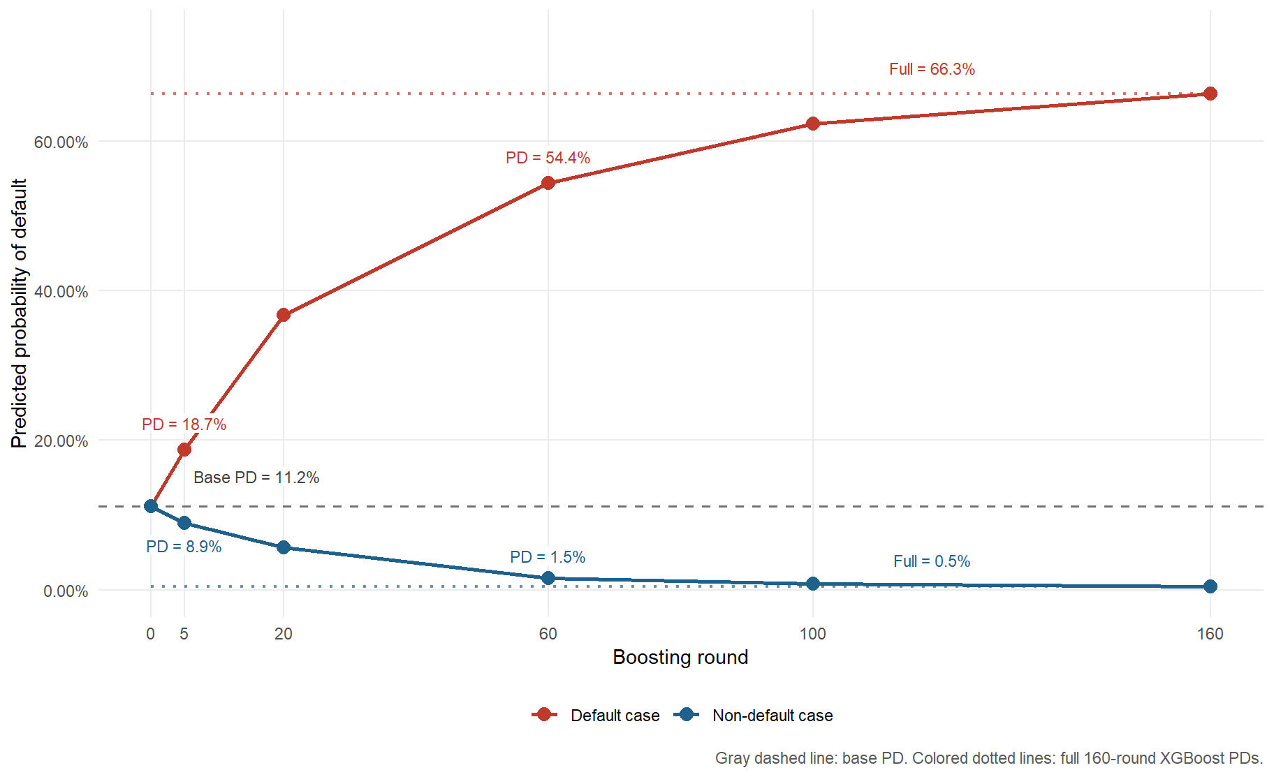
Figure 2.2: Predicted PD for two applicants as XGBoost boosting rounds accumulate.
The two cases show corrections in opposite directions under the same XGBoost specification. For the default case, the predicted PD moves from 11.18% at round 0 to 66.29% at round 160. For the non-default case, it moves from the same base PD to 0.48%. The colored dotted lines are now convergence references in a precise sense. They are the full 160-round XGBoost predictions for the same applicants. These two individual examples are useful because the corrections go in the direction suggested by the observed outcomes, and the individual log-loss falls in both rows of the check table. Overall performance still has to be evaluated on the full test set, as we do later with AUC, Brier score, calibration, and payoff.
The selected checkpoints are for teaching. In applied modeling, the number of trees should be chosen with a validation rule, cross-validation, or early stopping. The analyst stops adding trees when additional rounds no longer improve out-of-sample performance, or when the improvement is too small to justify the added complexity.
In notation, the boosted model builds a score \(F_M(x)\) by adding trees one at a time:
where \(f_m(x)\) is tree \(m\), \(M\) is the number of boosting rounds, and \(\eta\) is the learning rate. For binary classification, this score is transformed into a probability of default through the logistic function:
\[
\hat{p}(x) = \frac{1}{1 + \exp[-F_M(x)]}.
\]
The model is therefore still producing a probability of default. What changes is how the score behind that probability is constructed.
The score \(F_M(x)\) is on the log-odds scale. A higher score means higher predicted default risk after the logistic transformation. The code objects follow the same notation. xgb_nrounds is \(M\), xgb_params$eta is \(\eta\), xgb_model stores the fitted trees \(f_m\), and predict(xgb_model, newdata = xgb_test) returns \(\hat p(x)\).
The learning rate is the step size of the boosting process. In this chapter, eta is 0.05. If a new tree proposes a score correction, XGBoost uses only a fraction of that correction before adding the next tree. Smaller steps make learning slower, but they often produce a more stable model because no single tree can change the score too aggressively. The model also uses shallow trees, subsampling, column sampling, and regularization to reduce overfitting.
In a logistic regression, interpretation begins with a small number of coefficients. In XGBoost, interpretation begins with the ensemble. Many small trees combine to produce a score. That makes the model less transparent by construction. We can still inspect how the model learns, which variables it uses, how variables affect predicted default probabilities, and how the final predictions behave under the same credit-risk metrics used in Chapter 1.
The settings table above is the specification used by the full model estimated below. The checkpoint exercise changes only the number of boosting rounds used for prediction.
The objective binary:logistic tells XGBoost that the outcome is binary and that predictions should be probabilities between 0 and 1. More specifically, the model is trained to reduce a binary log-loss objective. For one applicant, the loss can be written as:
where \(y_i\) is 1 for default and 0 for no default, and \(\hat p_i\) is the predicted probability of default. This loss penalizes confident wrong probabilities heavily. If a borrower defaults and the model assigns a very low probability of default, the loss is large. If a borrower does not default and the model assigns a very high probability of default, the loss is also large. In code, objective = "binary:logistic" and eval_metric = c("logloss", "auc") connect this mathematical objective to the XGBoost estimation.
The maximum depth limits how complex each individual tree can be. The learning rate controls how strongly each tree contributes. Subsampling and column sampling make the model less dependent on any one subset of rows or variables. These choices are part of the model design and have computational consequences.
The financial interpretation is simple even if the algorithm is more complex. XGBoost is still trying to rank applicants by default risk and assign a usable PD. The extra machinery has value only if it improves those credit decisions out of sample.
2.5 Estimating the final XGBoost model
The previous sections prepared the XGBoost matrices and inspected how boosting rounds change predictions for selected applicants. We now estimate the final XGBoost model used in the benchmark. The objects xgb_train, xgb_test, xgb_train_label, and xgb_test_label already contain the encoded training and test data. The settings xgb_params and xgb_nrounds are the same settings used in the checkpoint exercise.
The estimation happens in the call to xgboost::xgb.train(). The inputs to that call identify what is being learned, from which data, and for how many boosting rounds. The printed training log is suppressed with verbose = 0 so the book output stays compact, but the model still stores the final fitted trees and the evaluation history.
Code
xgb_estimation_inputs <-data.frame(Argument =c("params = xgb_params","data = xgb_train","nrounds = xgb_nrounds","watchlist = list(train = xgb_train, test = xgb_test)","verbose = 0" ),Role =c("Objective, evaluation metrics, learning rate, depth, regularization, and sampling choices.","Encoded training matrix with the observed default labels.","Number of boosted trees added to the score.","Training and test matrices used to store diagnostic metrics during estimation.","Suppresses console printing; it does not change the estimated model." ),check.names =FALSE)knitr::kable( xgb_estimation_inputs,caption ="Inputs used by the XGBoost estimation call.",row.names =FALSE)
Inputs used by the XGBoost estimation call.
Argument
Role
params = xgb_params
Objective, evaluation metrics, learning rate, depth, regularization, and sampling choices.
data = xgb_train
Encoded training matrix with the observed default labels.
nrounds = xgb_nrounds
Number of boosted trees added to the score.
watchlist = list(train = xgb_train, test = xgb_test)
Training and test matrices used to store diagnostic metrics during estimation.
verbose = 0
Suppresses console printing; it does not change the estimated model.
The object xgb_model stores the fitted boosted trees. The object pred_xgb stores one predicted default probability for each applicant in the test set.
After this chunk, the model has been estimated. The next table makes the fitted object visible. The most important out-of-sample quantities are the test-set predictions, test AUC, and test Brier score. The training metrics are useful as diagnostics, but they are not the final criterion for credit-scoring performance.
The fitted object is valuable because it produces applicant-level PDs. The next two figures make those final predictions visible. The first figure compares the final PD distributions from the full logistic model and XGBoost. The second figure compares each XGBoost PD with the full logistic-model PD from Chapter 1 for the same test-set applicant, with separate panels for observed defaults and non-defaults.
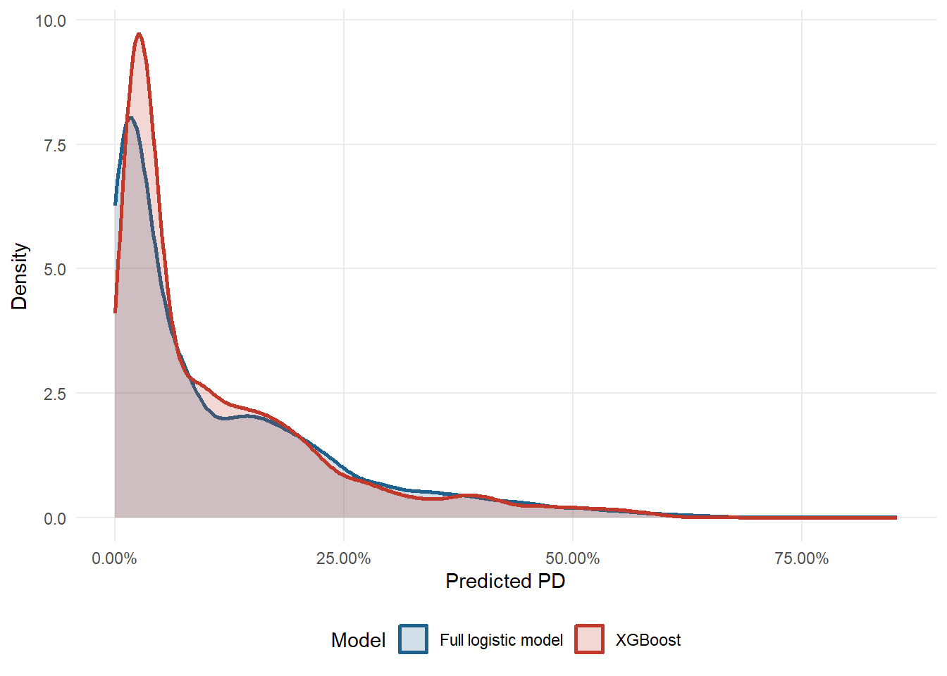
Figure 2.3: Final predicted PD distributions for the full logistic model and XGBoost.
Both models assign low PDs to many applicants, and the right tail is where the comparison becomes informative. The median PD is 6.18% for logi_full and 6.01% for XGBoost. At the 90th percentile, the corresponding values are 29.23% and 27.32%. At the 99th percentile, they are 54.00% and 52.77%. The plot therefore asks a credit-scoring question. Does the challenger model merely reproduce the logistic score, or does it redistribute applicants across the risk scale in a way that may change approvals, rejections, and expected losses?
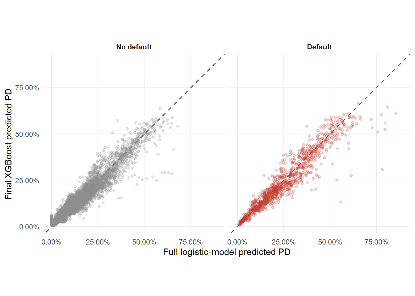
Figure 2.4: Full logistic-model PDs compared with final XGBoost PDs by observed outcome.
The dashed line is the equal-PD line. Points above the line are applicants for whom XGBoost assigns a higher PD than the logistic benchmark; points below the line receive a lower XGBoost PD. Separating the panels by observed outcome makes the comparison easier to read. Among applicants who defaulted, XGBoost assigns a higher PD than logi_full to 39.91% of cases. Their median PD moves from 22.48% under logi_full to 20.97% under XGBoost. Among applicants who repaid, XGBoost assigns a lower PD than logi_full to 45.06% of cases. Their median PD moves from 4.82% to 4.87%. The visual conclusion is mixed. XGBoost changes the risk ranking locally, while the panels do not show a uniform shift in the desired direction for all realized defaults and non-defaults. This prepares the reader for the broader evidence below. AUC, calibration, bad rates, and payoff must decide whether those local changes improve the credit policy.
The model was estimated with shallow trees and a moderate number of boosting rounds. The checkpoint exercise followed individual applicants; the learning curve below evaluates aggregate performance across the training and test sets. We re-estimate the model at selected boosting rounds and calculate AUC on both samples. The next code builds the data used in the learning-curve figure.
ggplot(xgb_learning_curve, aes(x = rounds, y = auc, color = series)) +geom_line(linewidth =1) +geom_point(size =2) +scale_color_manual(values =c("Train AUC"="steelblue","Test AUC"="firebrick")) +labs(x ="Boosting round", y ="AUC", color ="Series") +theme_minimal() +theme(legend.position ="bottom")
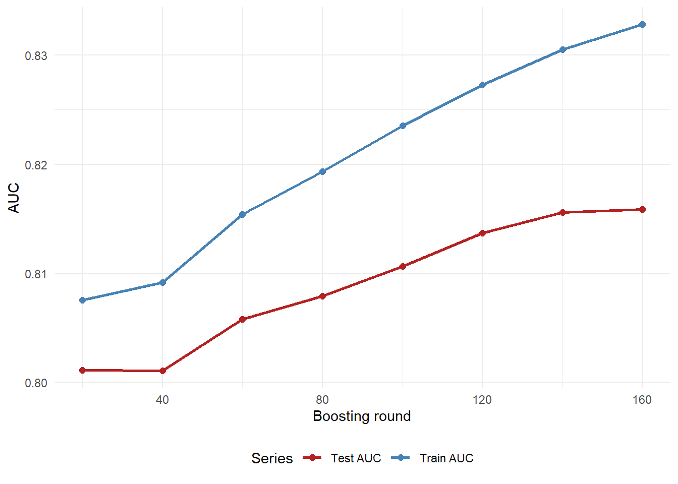
Figure 2.5: XGBoost learning curve: test AUC with train AUC as a diagnostic reference.
The red test-AUC line is the main out-of-sample quantity in Figure 2.5. The blue train-AUC line is included as a diagnostic reference. A direct overfitting check has two parts. First, inspect whether test AUC deteriorates as more boosting rounds are added. Second, compare how far train AUC sits above test AUC at the final model.
Code
xgb_overfitting_check <-data.frame(Check =c("Best test AUC in the grid","Final test AUC","Change in test AUC from previous checkpoint","Final train AUC","Final train-test AUC gap","Test AUC declines after its best checkpoint?" ),Value =c(paste0(fmt_num(xgb_best_test_row$auc, 4)," at ",fmt_int(xgb_best_test_row$rounds)," rounds" ),fmt_num(xgb_final_test_auc, 4),fmt_num(xgb_test_auc_last_change, 4),fmt_num(xgb_final_train_auc, 4),fmt_num(xgb_final_auc_gap, 4),ifelse(xgb_test_auc_declines_after_best, "Yes", "No") ),Reading =c("Highest out-of-sample ranking result among the inspected checkpoints.","Ranking result for the model used in the chapter.","Positive values mean the last added rounds still improved test ranking.","In-sample ranking result.","Larger gaps call for validation, calibration, and monitoring.","A decline would be direct evidence that additional rounds are hurting test ranking." ),check.names =FALSE)knitr::kable( xgb_overfitting_check,caption ="Direct overfitting diagnostic from the XGBoost learning curve.",row.names =FALSE)
Direct overfitting diagnostic from the XGBoost learning curve.
Check
Value
Reading
Best test AUC in the grid
0.8158 at 160 rounds
Highest out-of-sample ranking result among the inspected checkpoints.
Final test AUC
0.8158
Ranking result for the model used in the chapter.
Change in test AUC from previous checkpoint
0.0003
Positive values mean the last added rounds still improved test ranking.
Final train AUC
0.8328
In-sample ranking result.
Final train-test AUC gap
0.0170
Larger gaps call for validation, calibration, and monitoring.
Test AUC declines after its best checkpoint?
No
A decline would be direct evidence that additional rounds are hurting test ranking.
In this run, the best inspected test AUC occurs at 160 boosting rounds, and the final test AUC is 0.8158. The last inspected movement in test AUC is 0.0003. The training AUC is 0.8328, so the final train-test gap is 0.0170. The evidence therefore supports a cautious reading. The selected grid does not show test-AUC deterioration after the best checkpoint, while the train-test gap still deserves validation and monitoring.
The curve is a diagnostic. A careful optimization workflow would use cross-validation or a separate validation set to select the number of rounds and other hyperparameters, and only then evaluate the final model on the test set.
The distinction between the teaching workflow and a production workflow is important. This chapter uses the same test set repeatedly because the objective is to make the comparison visible. In production, the analyst should separate three tasks. Fit the model, choose tuning parameters, and report final performance.
Code
xgb_validation_workflow <-data.frame(Stage =c("Training","Validation or cross-validation","Final holdout test","Monitoring after deployment" ),`What it answers`=c("Which patterns can the model learn from historical applications?","Which hyperparameters give stable out-of-sample behavior?","How well does the chosen model perform on untouched borrowers?","Do ranking, calibration, bad rates, and approval patterns remain stable over time?" ),`Typical XGBoost checks`=c("Fit shallow boosted trees with regularization and subsampling.","Tune rounds, depth, learning rate, minimum child weight, subsampling, and calibration.","Report AUC, Brier score, calibration, bad rates, and payoff once.","Track drift, overrides, calibration decay, fairness checks, and reject-inference issues." ),check.names =FALSE)knitr::kable( xgb_validation_workflow,caption ="Teaching workflow versus production validation for XGBoost credit scoring.",row.names =FALSE)
Teaching workflow versus production validation for XGBoost credit scoring.
Stage
What it answers
Typical XGBoost checks
Training
Which patterns can the model learn from historical applications?
Fit shallow boosted trees with regularization and subsampling.
Validation or cross-validation
Which hyperparameters give stable out-of-sample behavior?
How well does the chosen model perform on untouched borrowers?
Report AUC, Brier score, calibration, bad rates, and payoff once.
Monitoring after deployment
Do ranking, calibration, bad rates, and approval patterns remain stable over time?
Track drift, overrides, calibration decay, fairness checks, and reject-inference issues.
The learning curve should therefore be read as a diagnostic rather than a full tuning exercise. If test AUC rose and then deteriorated, the analyst would stop adding trees. If validation calibration worsened while AUC improved, the analyst might keep the ranking model and recalibrate the probabilities before using them for pricing or provisioning.
XGBoost prediction range and test-set performance summary.
Quantity
Value
Minimum predicted PD
0.48%
Median predicted PD
6.01%
Maximum predicted PD
66.29%
AUC
0.8158
Brier score
0.0826
The XGBoost model returns predicted probabilities of default, just like the logistic model. In code, those probabilities are stored in pred_xgb; mathematically, they are the \(\hat p_i\) values used by the same evaluation equations from Chapter 1. Therefore, all the credit-risk tools developed in Chapter 1 still apply. These include cutoffs, acceptance rates, bad rates, calibration, Brier score, and net payoff.
The prediction range table should be read as a risk-segmentation summary. The minimum, median, and maximum predicted PD tell us how widely the model spreads applicants across the risk scale. A model that assigns nearly the same PD to everyone would have little value for screening, even if that average PD were reasonable. A useful scoring model must separate applicants enough to support different decisions.
2.6 Interpreting XGBoost
The main risk with XGBoost is practical. The model is easier to use than to understand. We therefore need several complementary views of the model. Each plot answers one specific question, and the collection helps us understand what the model uses, how it moves predictions, and whether those movements are acceptable for credit decisions.
The first view is feature importance. XGBoost can report which encoded variables are used most often and most effectively in the ensemble.
Code
xgb_importance |>slice_max(Gain, n =12) |>mutate(Feature =reorder(Feature, Gain)) |>ggplot(aes(x = Gain, y = Feature)) +geom_col(fill ="steelblue") +labs(x ="Gain", y ="Feature") +theme_minimal()
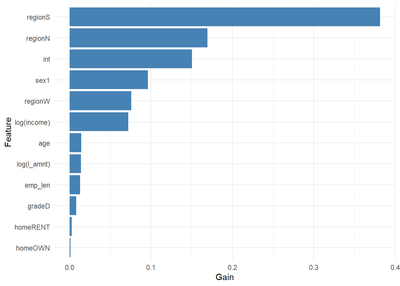
Figure 2.6: XGBoost feature importance.
Gain measures how much a feature contributes to improving the model’s splits. It tells us that the model uses that feature to reduce prediction error. In this run, the three largest Gain variables are regionS, regionN, int. That result should be read as a model-use ranking. The model is finding useful segmentation in those encoded inputs, especially for separating applicants into different predicted-risk groups. Direction and local interpretation require another tool.
This distinction is central in credit scoring. A high-Gain variable is important for prediction. The plot leaves two questions open. Do larger values of that variable increase or decrease default risk, and is the effect the same for every borrower? Gain therefore maps where the model is looking. Applicant-level interpretation requires additional tools.
SHAP-style contributions provide a second view. For each observation, XGBoost can decompose the model score into contributions from the encoded variables plus a baseline term:
The contributions \(\phi_{ij}\) are on the model-score scale before the logistic transformation. A positive contribution increases the score and therefore pushes the prediction toward higher default risk; a negative contribution lowers the score and pushes the prediction toward lower default risk. In code, xgb_shap <- predict(xgb_model, newdata = xgb_test, predcontrib = TRUE) creates the contribution values. The BIAS column corresponds to \(\phi_0\), and the other columns correspond to the feature contributions \(\phi_{ij}\).
Code
xgb_shap_importance |>slice_max(mean_abs_shap, n =12) |>mutate(feature =reorder(feature, mean_abs_shap)) |>ggplot(aes(x = mean_abs_shap, y = feature)) +geom_col(fill ="darkorange") +labs(x ="Mean absolute contribution", y ="Feature") +theme_minimal()
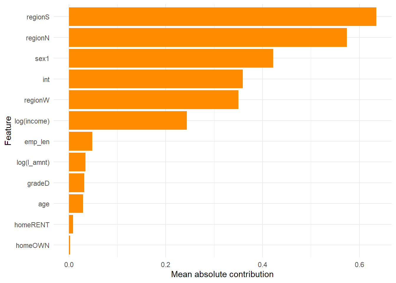
Figure 2.7: Average absolute XGBoost contribution by feature.
This plot is closer to an explanation of prediction behavior. A high average absolute contribution means that the feature often moves predictions away from the baseline. In this run, the largest average absolute contributions come from regionS, regionN, sex1. The careful reading is directional. These variables often move the XGBoost score materially, sometimes upward and sometimes downward, depending on the applicant. Direction requires applicant-level contributions or partial dependence.
For credit work, the useful reading is layered. Feature importance tells us where the model finds predictive structure. SHAP-style magnitudes tell us which encoded borrower or loan signals materially move predictions. The analyst still has to check whether those signals are defensible for credit decisions, stable out of sample, and acceptable under governance, fairness, and adverse-action requirements.
We can make this more concrete by returning to the same first test-set applicant used in Chapter 1, whom we called John Doe. We also include the two applicants used in the XGBoost checkpoint exercise above. This makes the table a bridge between the chapter’s worked examples and the final model comparison.
The table compares the full logistic model, the single tree, and XGBoost for three concrete applicants. All values are probabilities of default, so they can be compared directly within each applicant. What differs is the way each model arrives at that probability. The logistic model uses a coefficient equation, the single tree uses a terminal-leaf default rate, and XGBoost uses the sum of many tree contributions.
For John Doe specifically, the observed outcome is loan_st = 0, meaning no default. The two selected checkpoint cases show a wider range of behavior because one is a realized default and the other is a realized non-default. The table is a probability comparison rather than a three-case accuracy test. A single realized outcome is binary, while a PD is a forecast of risk before repayment is observed. The general comparison still has to come from the full test set.
For XGBoost, the local explanation follows the score equation introduced above:
The next table verifies the mechanics. The baseline plus all feature contributions gives the XGBoost score \(F_i\). Applying the logistic transformation to that score gives the same probability returned by predict(xgb_model, ...).
Reconstructing John Doe’s XGBoost score and predicted PD.
Component
Value
baseline score
-2.0892
sum of feature contributions
-1.3839
total score F_i
-3.4731
logistic transformation of F_i
3.01%
direct XGBoost prediction
3.01%
The largest local contributions for John Doe are:
Code
john_xgb_contribution_table |>mutate(contribution =fmt_num(contribution, 4)) |> knitr::kable(caption ="Largest local XGBoost contributions for John Doe.",row.names =FALSE )
Largest local XGBoost contributions for John Doe.
feature
contribution
regionS
-0.7559
sex1
-0.7388
regionW
-0.4210
regionN
0.2784
log(income)
0.2685
gradeD
-0.0242
emp_len
0.0176
int
-0.0078
A positive contribution increases John Doe’s XGBoost score and therefore increases the predicted probability of default. A negative contribution lowers the score and therefore lowers the predicted probability of default. These values are score-scale contributions before the logistic transformation, so the contribution table should be read together with the score reconstruction table.
For this applicant, the reconstructed score is -3.4731. Applying the logistic transformation gives a predicted PD of 3.01%, which matches the direct XGBoost prediction. This numerical check is important because it connects the local explanation table to the actual probability used in the lending decision.
The third view is partial dependence. Here we change one variable at a time and average the model’s predicted probability over the test set. This gives an approximate picture of how the model behaves as that variable changes, while the empirical distribution of the other variables is kept in the background.
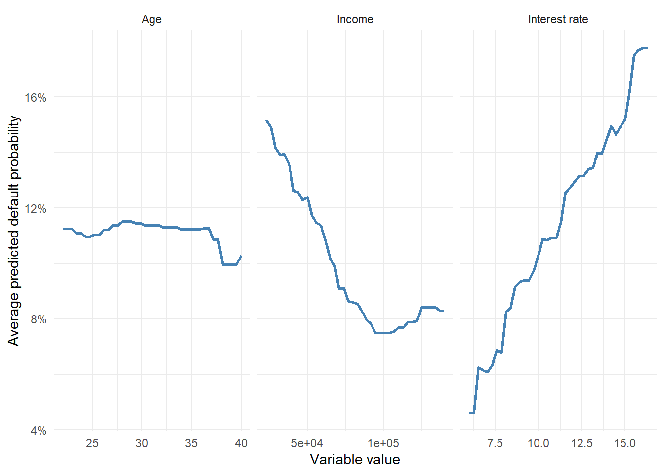
Figure 2.8: Partial dependence of XGBoost predicted default probability.
Partial dependence should be read as model behavior rather than causal evidence. Changing a borrower’s age, income, or interest rate in this plot shows how the fitted model’s predictions move when we vary one input while averaging over the observed test set. This is useful because it makes part of the model’s internal behavior visible.
A useful way to read the plot is to imagine a controlled model exercise. For the interest-rate panel, for example, we repeatedly give the model the same test-set borrowers but replace the interest rate by one value on the horizontal axis. We then average the predicted PDs. The curve therefore answers a model question. How does the fitted XGBoost score respond when this input changes across the observed range?
The panels give three different readings. In the interest-rate panel, the average predicted PD rises from 4.60% at the lowest inspected rate to 17.75% at the highest inspected rate. In the income panel, the average predicted PD moves from 15.16% at the low-income end to 8.29% at the high-income end. The age panel is much flatter, ranging from 9.96% to 11.51% across the inspected ages. This is exactly the type of reading an analyst needs. The model is sensitive to some credit signals and much less sensitive to others.
The interpretation strategy is therefore layered:
Feature importance tells us what the model uses.
SHAP-style contributions tell us what moves predictions.
Partial dependence shows how predicted risk changes across selected variables.
Calibration and performance metrics tell us whether the predictions behave well out of sample.
This is how XGBoost can be made more transparent by inspection, while logistic regression remains more transparent by construction.
2.7 Benchmarking against logistic regression
We can now compare the tree-based models with the logistic benchmark. The comparison is intentionally based on the same criteria used in Chapter 1. This avoids changing the rules after changing the model.
Code
model_metrics_table <- model_metrics |>mutate(auc =fmt_num(auc, 4),brier_score =fmt_num(brier_score, 4),brier_skill =fmt_num(brier_skill, 4) )knitr::kable( model_metrics_table,caption ="Out-of-sample performance of the credit-scoring models.",row.names =FALSE)
Out-of-sample performance of the credit-scoring models.
model
auc
brier_score
brier_skill
logi_full
0.8213
0.0822
0.1559
single_tree
0.6590
0.0882
0.0938
xgboost
0.8158
0.0826
0.1523
constant default rate
NA
0.0974
0.0000
AUC measures ranking ability. Do defaulting borrowers tend to receive higher predicted probabilities than non-defaulting borrowers? The Brier score measures probability error. Are the predicted probabilities numerically close to the observed outcomes? Brier skill expresses improvement relative to the constant default-rate benchmark. A positive value means the model improves on assigning every applicant the same default probability. In code, model_metrics collects these three criteria for the logistic benchmark, the single tree, and XGBoost.
In this run, the highest AUC belongs to logi_full with AUC 0.8213. The lowest Brier score belongs to logi_full with Brier score 0.0822. These two criteria may point to the same model or to different models because they answer different questions. AUC asks whether the ranking is good. Brier score asks whether the probabilities are numerically close to the realized default outcomes.
The results are useful precisely because they are mixed. XGBoost is a more flexible model class. In this specification, it is close to the logistic benchmark, with no dramatic improvement on every metric. The challenger-model reading is therefore conservative. XGBoost has AUC 0.8158 versus 0.8213 for logi_full, and Brier score 0.0826 versus 0.0822. Under the payoff rule used below, the best XGBoost strategy differs from the best logistic strategy by $1. A modern algorithm earns its place only when the ranking, probability quality, and decision consequences improve together.
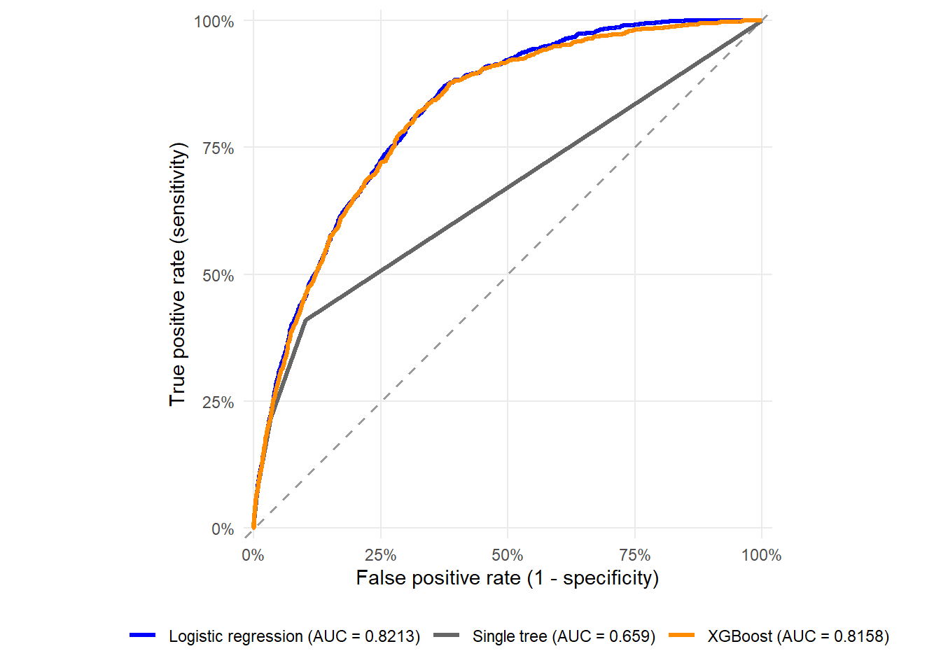
Figure 2.9: ROC curves: logistic regression, single tree, and XGBoost.
The ROC comparison focuses on ranking. If the XGBoost curve lies above the logistic curve, the boosted model is doing a better job ranking defaulting borrowers above non-defaulting borrowers. The final lending strategy still depends on cutoffs, costs, and calibration.
This is the same logic as in Chapter 1. ROC curves ignore the size of the predicted PDs and focus on ordering. If one applicant receives 18% and another receives 4%, ROC only cares that the higher-risk applicant is ranked above the lower-risk applicant. A lending policy still has to decide where to put the cutoff and what loss is attached to accepting a borrower who defaults.
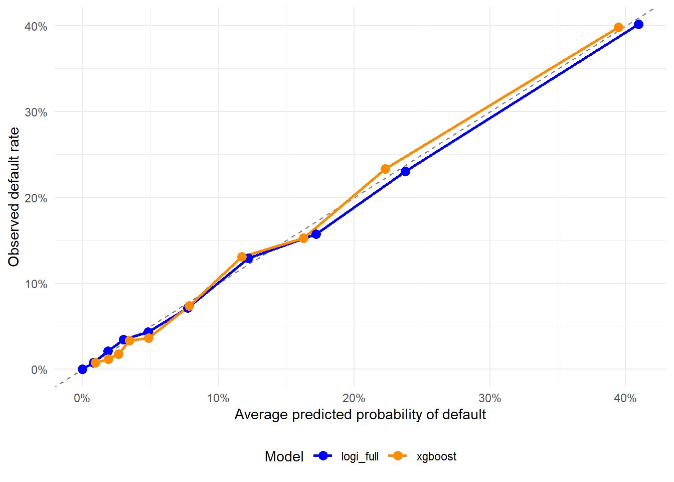
Figure 2.10: Calibration by decile: logistic regression and XGBoost.
Calibration is important because both models produce probabilities of default. A model can rank applicants well and still produce probabilities that are too high or too low. If the calibration curve is far from the dashed line, we should be cautious about interpreting the raw predicted values as literal probabilities.
The dashed line is the ideal reference. A point near 10% on both axes means that applicants assigned an average PD near 10% defaulted about 10% of the time in that decile. A point above the line means realized defaults were higher than predicted in that group. A point below the line means realized defaults were lower than predicted. This plot therefore checks whether the PD numbers can be read as probabilities as well as ranks.
If a flexible model ranks applicants well while its probabilities need improvement for pricing, provisioning, or stress testing, a common workflow is to keep the ranking model and recalibrate its predicted probabilities using a separate validation sample. Methods such as logistic calibration, sometimes called Platt scaling, or isotonic regression are designed for that purpose. Recalibration is outside this chapter, and the calibration plot tells us whether such a step may be needed before treating the predicted values as operational probabilities of default.
Code
strategy_comparison |>ggplot(aes(x = accept_rate, y = bad_rate, color = model)) +geom_line(linewidth =1.1) +geom_point(size =2) +scale_color_manual(values =c("logi_full"="blue","single_tree"="gray40","xgboost"="darkorange")) +scale_x_continuous(labels = scales::percent_format(accuracy =1)) +scale_y_continuous(labels = scales::percent_format(accuracy =1)) +labs(x ="Acceptance rate", y ="Bad rate", color ="Model") +theme_minimal() +theme(legend.position ="bottom")
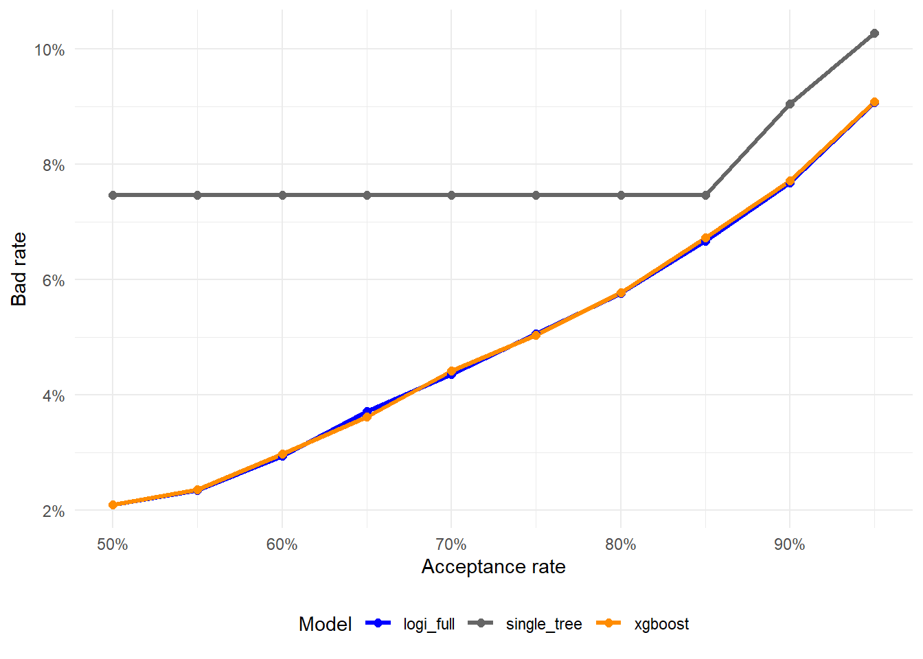
Figure 2.11: Bad rate by acceptance rate: logistic regression, single tree, and XGBoost.
This plot translates model predictions into lending strategy. In code, strategy_comparison stores the acceptance rate, cutoff, accepted defaults, bad rate, and net payoff for each model. At a fixed acceptance rate, the preferred model is the one with the lower bad rate. This is often more intuitive for credit risk than raw accuracy because it focuses on the loans actually accepted by the bank.
At an 80% acceptance rate, the lowest bad rate in this run is produced by logi_full, with bad rate 5.76%. This means that among the applicants accepted by that model at that acceptance rate, 5.76% defaulted in the historical test set. The comparison is operational. It asks which score gives the cleaner accepted portfolio when the bank wants to approve the same share of applicants.
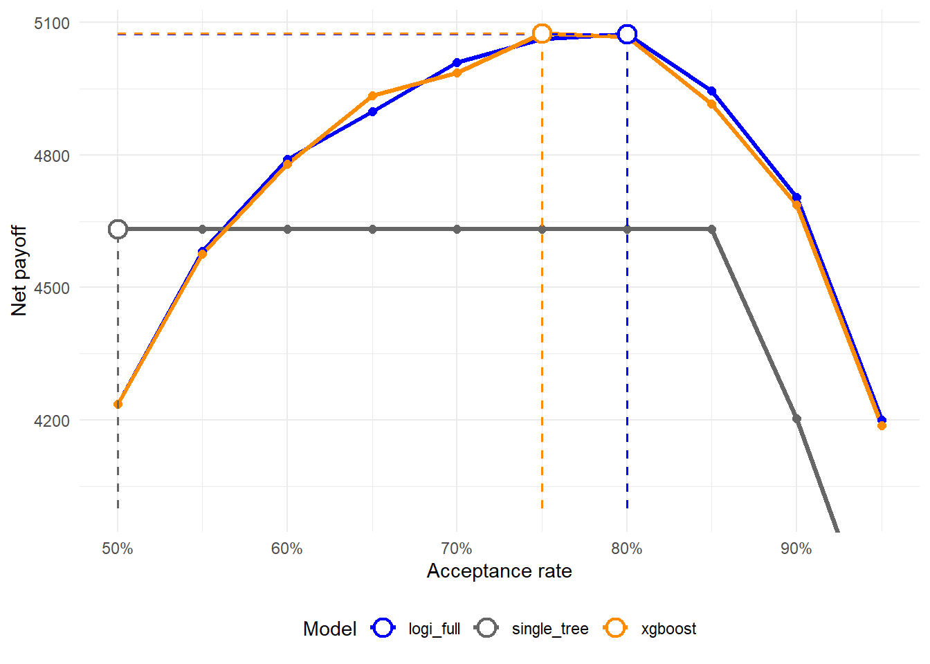
Figure 2.12: Net payoff by acceptance rate: logistic regression, single tree, and XGBoost.
The net payoff curve uses the same pedagogical assumption introduced in Chapter 1. Accepting a good loan has payoff $1, accepting a default has cost $5, and rejecting an application has payoff $0. The dashed guides mark the maximum net payoff reached by each model. Under this assumption, the best model may differ from the model with the highest AUC. The selected model is the one that produces better decisions under the payoff rule.
The payoff curve is the most direct bridge from statistical scoring to a business decision. For every acceptance rate, the cutoff determines which applicants are accepted. The realized defaults among those accepted loans create costs, and the realized non-defaults create gains. Under the assumed payoff rule, the best observed strategy in this comparison is xgboost, with net payoff $5,075 at an acceptance rate of 75%.
The payoff calculation for that row is the same one used in Chapter 1:
This final table makes the comparison concrete. It shows the acceptance rate at which each model reaches its highest net payoff under the assumed cost structure. In this run, XGBoost and logistic regression are very close. A reasonable analyst conclusion is to keep XGBoost as a challenger model. It is valuable because it tests whether nonlinear segmentation improves credit decisions, while the final policy should still be chosen from the combined evidence on AUC, calibration, bad rates, and payoff. The same decision framework shows where the flexible model changes the lending strategy and where it gives a similar answer.
2.8 What do we gain and what do we lose?
The comparison with logistic regression should be read as a model governance exercise. Both approaches estimate default probabilities through different mechanisms and require different checks.
Logistic regression is transparent by construction. Its coefficients have a clear mathematical interpretation in terms of log-odds and odds ratios. This makes it easier to audit, explain, and communicate. It is also easier to diagnose when the model form is too restrictive.
XGBoost is more flexible. It can capture nonlinear patterns and interactions without requiring the analyst to write those interactions into the formula. This can improve ranking, bad rates, or net payoff. That flexibility comes with responsibilities. Tuning, validation, calibration, and interpretation are required parts of model governance.
The main lesson is that a modern model becomes useful only after it improves the credit policy. A better model must still survive several questions:
Does it improve out-of-sample ranking?
Are its probabilities reasonably calibrated?
Does it reduce bad rates at relevant acceptance rates?
Does it improve net payoff under explicit business assumptions?
Can we explain the model well enough for governance and decision-making?
The same questions can be turned into an analyst checklist. In this chapter, the checklist has a specific interpretation. XGBoost is useful as a challenger because it tests whether nonlinear segmentation improves the credit policy. The model becomes a candidate for production only if the evidence is strong across several dimensions at the same time. Those dimensions are ranking, probability quality, cutoff behavior, economic payoff, and explainability.
Code
tree_governance_checklist <-data.frame(Check =c("Ranking","Probability quality","Cutoff decision","Economic consequence","Interpretability","Model governance" ),`Evidence used in this chapter`=c("ROC curve and AUC","Brier score and calibration by decile","Bad rate by acceptance rate","Net payoff under an explicit cost rule","Tree leaves, feature importance, SHAP-style contributions, and partial dependence","Training/test comparison and stated need for validation or cross-validation" ),`Production extension`=c("Validate ranking on a holdout sample and across time.","Recalibrate probabilities when the ranking is useful but PD levels are biased.","Choose cutoffs with business, risk-appetite, and compliance constraints.","Replace the teaching payoff with loan-level profitability, LGD, EAD, and funding costs.","Document drivers, adverse-action logic, stability, and fairness implications.","Use cross-validation, monitoring, challenger models, and periodic recalibration." ),check.names =FALSE)knitr::kable( tree_governance_checklist,caption ="Governance checklist for moving from a tree-based score to a credit policy.",row.names =FALSE)
Governance checklist for moving from a tree-based score to a credit policy.
Check
Evidence used in this chapter
Production extension
Ranking
ROC curve and AUC
Validate ranking on a holdout sample and across time.
Probability quality
Brier score and calibration by decile
Recalibrate probabilities when the ranking is useful but PD levels are biased.
Cutoff decision
Bad rate by acceptance rate
Choose cutoffs with business, risk-appetite, and compliance constraints.
Economic consequence
Net payoff under an explicit cost rule
Replace the teaching payoff with loan-level profitability, LGD, EAD, and funding costs.
Interpretability
Tree leaves, feature importance, SHAP-style contributions, and partial dependence
Document drivers, adverse-action logic, stability, and fairness implications.
Model governance
Training/test comparison and stated need for validation or cross-validation
Use cross-validation, monitoring, challenger models, and periodic recalibration.
XGBoost can be useful in credit scoring precisely because it gives us a stronger benchmark than a single logistic specification. It should be used as part of a disciplined workflow. The model may be complex, while the evaluation criteria must remain clear.
The disciplined workflow is the main takeaway of the chapter. First, define the credit decision. Second, estimate competing PD models on the same training information. Third, evaluate them on the same out-of-sample borrowers. Fourth, compare ranking, calibration, bad rates, and payoff together. A flexible model becomes valuable when it improves the decision problem rather than simply using a more advanced algorithm.