3 Robotrader in R
The previous chapter introduced the return objects used to compare assets, measure risk, and summarize price movements. This chapter keeps that foundation and adds a trading layer: prices and returns become lagged indicators, those indicators become predictors, and the resulting predictions are evaluated with a simple out-of-sample trading rule.
Stock price movements are influenced by a large number of factors, including market trends, economic indicators, company-specific news, liquidity, risk appetite and investor expectations. Predicting precise daily movements is a hard problem. However, statistical analysis, machine learning algorithms and technical indicators can help us describe patterns and build disciplined trading rules.
The purpose is pedagogical: moving averages are used to build features, estimate a classification model, and translate the classification into a trading signal. The model is presented for learning and should not be read as an investment recommendation. It is a compact example of the full workflow. The sequence is to download prices, calculate returns, engineer predictors, split the data in time order, estimate a model, evaluate out-of-sample accuracy, and finally test a simple trading rule.
The trading rules use the same timing discipline. Before the return for day \(t\) is known, the model uses information available through day \(t-1\) to predict whether day \(t\) will be Up or Down. The chapter then compares a conservative long/cash rule, an aggressive long/short rule, and the same long/short rule after trading and short-selling costs. This timing convention is essential because today’s close is excluded from the information set used to predict today’s close-to-close return.
The mathematical objects in the chapter are defined below.
\[ P_t = \text{closing price on day } t, \]
\[ r_t = \frac{P_t}{P_{t-1}} - 1, \]
\[ x_{t-1} = \left( \text{SMA}_{5,t-1}, \text{SMA}_{10,t-1}, \text{SMA}_{15,t-1}, \text{SMA}_{20,t-1} \right), \]
and
\[ d_t = \begin{cases} \text{Up}, & r_t > 0,\\ \text{Down}, & r_t \leq 0. \end{cases} \]
The classification model estimates a rule
\[ \hat{g}(x_{t-1}) \in \{\text{Down}, \text{Up}\}. \]
The trading rule then converts the predicted class into a position and a strategy return. This bridge should remain visible: prices become returns, returns become labels, lagged moving averages predict labels, and predictions become trading positions.
3.1 Download the data
The chosen period includes both training and test data.
The first rows verify the downloaded structure.
# A tibble: 6 × 8
  symbol date        open  high   low close    volume adjusted
  <chr>  <date>     <dbl> <dbl> <dbl> <dbl>     <dbl>    <dbl>
1 AAPL   2021-01-04  134.  134.  127.  129. 143301900     126.
2 AAPL   2021-01-05  129.  132.  128.  131.  97664900     127.
3 AAPL   2021-01-06  128.  131.  126.  127. 155088000     123.
4 AAPL   2021-01-07  128.  132.  128.  131. 109578200     127.
5 AAPL   2021-01-08  132.  133.  130.  132. 105158200     128.
6 AAPL   2021-01-11  129.  130.  128.  129. 100384500     125.
The closing price is kept, and daily returns are calculated. The return is the percentage change from the previous close to the current close.
The formula implemented in the code is
\[ r_t = \frac{P_t-P_{t-1}}{P_{t-1}} = \frac{P_t}{P_{t-1}}-1. \]
If \(r_t=0.01\), the stock increased by 1% from the previous close. If \(r_t=-0.01\), the stock decreased by 1%.
Code
# A tibble: 6 × 4
  date       close    volume   return
  <date>     <dbl>     <dbl>    <dbl>
1 2021-01-05  131.  97664900  0.0124
2 2021-01-06  127. 155088000 -0.0337
3 2021-01-07  131. 109578200  0.0341
4 2021-01-08  132. 105158200  0.00863
5 2021-01-11  129. 100384500 -0.0232
6 2021-01-12  129.  91951100 -0.00140
3.2 Visualize the data
The red line splits the training and test data. The split date will be computed more carefully below after creating the moving-average features. For now, the line gives the same visual idea as the later train/test split.
Code
visual_split <- as.Date("2022-08-17")

prices %>%
  ggplot(aes(date, close)) +
  geom_line(color = "black", linewidth = 0.5) +
  geom_vline(xintercept = visual_split, color = "red", linetype = 2) +
  annotate("text", x = as.Date("2021-11-01"), y = 120,
           label = "Directional trading is difficult.",
           color = "black") +
  labs(x = "Date", y = "Close price") +
  scale_y_continuous(labels = scales::dollar)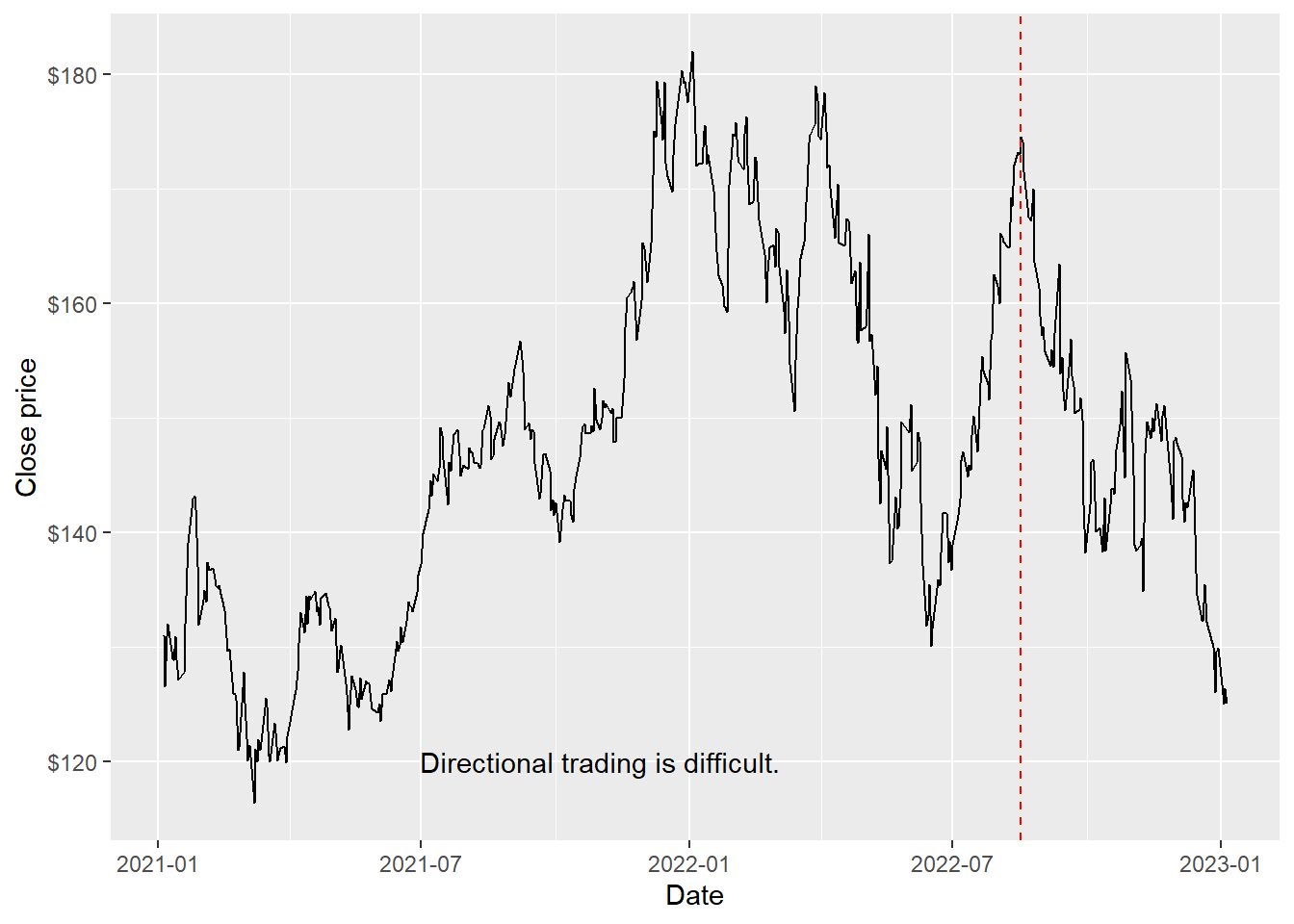
The series has a clear change in tone after the visual split: the test window starts during a weaker price environment. This matters because the buy-and-hold benchmark will be exposed to that decline, while the robo trader can reduce or reverse exposure when it predicts Down.
These are the corresponding daily returns.
# A tibble: 10 × 2
   date         return
   <date>        <dbl>
 1 2021-01-05  0.0124
 2 2021-01-06 -0.0337
 3 2021-01-07  0.0341
 4 2021-01-08  0.00863
 5 2021-01-11 -0.0232
 6 2021-01-12 -0.00140
 7 2021-01-13  0.0162
 8 2021-01-14 -0.0151
 9 2021-01-15 -0.0137
10 2021-01-19  0.00543
The density plot summarizes the distribution of daily returns.
Code
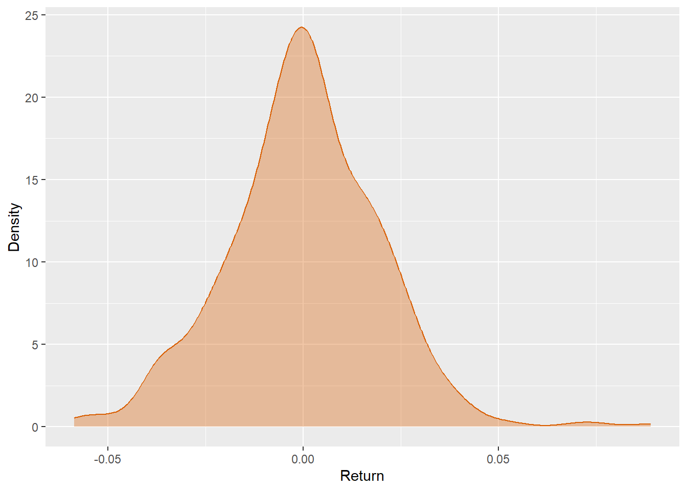
Most daily returns are concentrated close to zero, which is typical for daily stock data. The wider parts of the density show that a small number of days can produce meaningfully larger gains or losses. A directional model has to work in this noisy environment, where many observations are small and hard to classify.
The empirical density can be compared with a simulated normal distribution.
Code
normal_returns <- tibble(
  return = rnorm(100000, mean(prices$return), sd(prices$return))
)

ggplot() +
  geom_density(data = prices, aes(return, fill = "Return"),
               alpha = 0.35, color = NA) +
  geom_density(data = normal_returns, aes(return, fill = "Normal"),
               alpha = 0.35, color = NA) +
  scale_fill_manual(values = c("Return" = "#D95F02", "Normal" = "#1B9E77")) +
  labs(x = "Return", y = "Density", fill = "")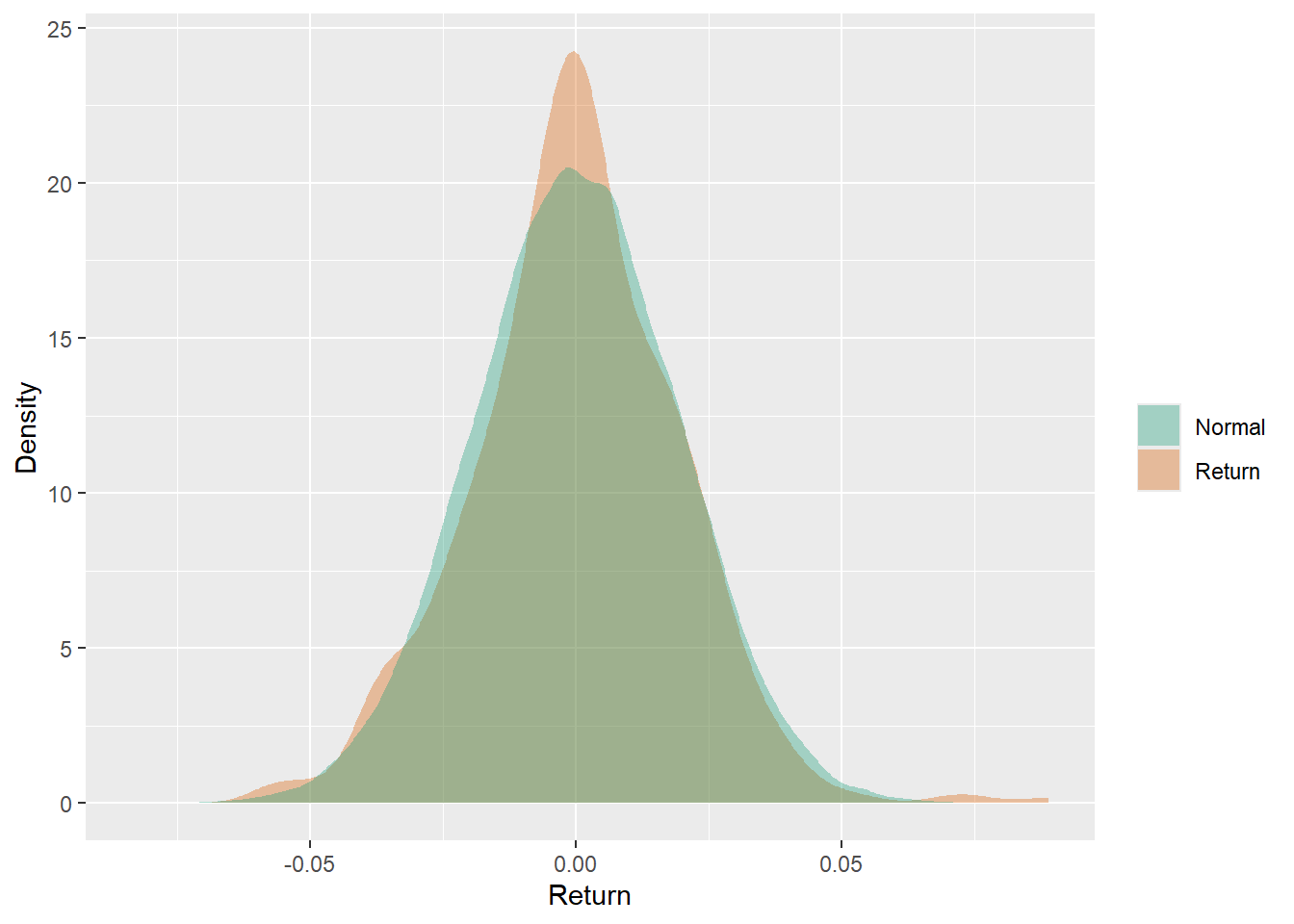
The empirical return distribution is more irregular than the simulated normal benchmark. This visual comparison is a reminder that daily returns can have asymmetry and tail behavior that a simple normal approximation may smooth away. For trading, those tail days can dominate cumulative performance.
The same returns can be separated into positive and negative days across the training and test periods.
Code
prices %>%
  mutate(direction = if_else(return > 0, "Positive", "Negative")) %>%
  ggplot(aes(date, return, fill = direction)) +
  geom_col(width = 1) +
  geom_vline(xintercept = visual_split, color = "black", linetype = 2) +
  scale_fill_manual(values = c("Positive" = "#1B9E77", "Negative" = "#D95F02")) +
  labs(x = "Date", y = "Return", fill = "")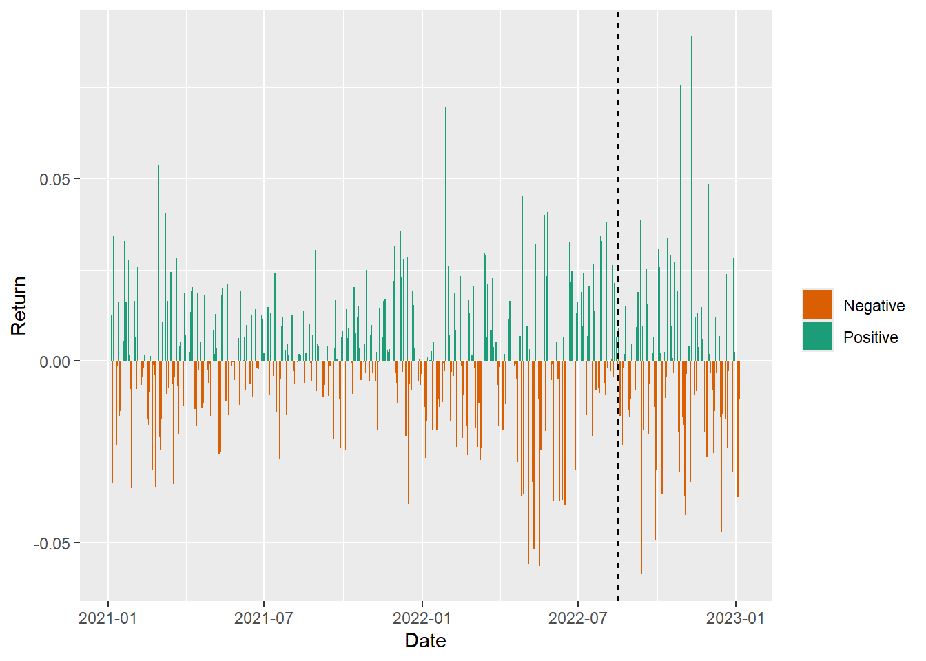
The bars show that positive and negative days arrive in clusters and alternate frequently. The test period includes several negative stretches, which creates an environment where avoiding exposure, or taking short exposure, can matter more than slightly improving average classification accuracy.
The test set daily returns are isolated using the visual split, and cumulative returns are calculated under a one-dollar initial investment with reinvested gains and losses.
For buy-and-hold, the value of one dollar after day \(t\) is
\[ C_t^{BH} = \prod_{i=1}^{t}(1+r_i). \]
This is a useful benchmark because it asks whether the trading rule adds value relative to simply holding the stock over the same period.
Code
# A tibble: 6 × 5
  date       close   volume   return cumulative_return
  <date>     <dbl>    <dbl>    <dbl>             <dbl>
1 2022-08-17  175. 79542000  0.00878             1.01
2 2022-08-18  174. 62290100 -0.00229             1.01
3 2022-08-19  172. 70346300 -0.0151              0.991
4 2022-08-22  168. 69026800 -0.0230              0.968
5 2022-08-23  167. 54147100 -0.00203             0.966
6 2022-08-24  168. 53841500  0.00179             0.968
The benchmark can be plotted directly.
Code
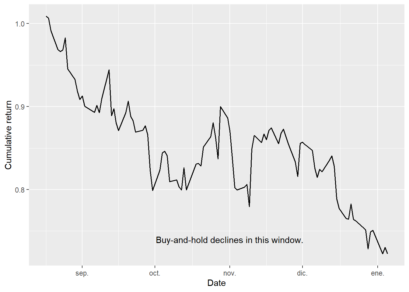
The buy-and-hold benchmark loses value during the test window. This gives the robo trader a concrete benchmark: a useful rule should either avoid part of the decline or benefit from correctly identified down days.
3.3 Simple moving averages
As technical analysis suggests, simple moving averages can be used as a tool to summarize recent price behavior. A moving average places the current price relative to its recent history.
For a window length \(n\), the simple moving average is
\[ \text{SMA}_{n,t} = \frac{1}{n}\sum_{j=0}^{n-1}P_{t-j}. \]
The 5-day average reacts quickly to recent price changes. The 20-day average reacts more slowly. The model receives several windows so it can compare short and medium-term price behavior.
The windows 5, 10, 15 and 20 are deliberately simple. They represent roughly one trading week, two trading weeks, three trading weeks and one trading month. They are not selected by looking at the test return. The purpose is to give the model a small, readable set of short- and medium-horizon trend summaries.
The code calculates 5, 10, 15 and 20 day moving averages.
The first observations are lost when computing moving averages because the rolling window needs enough previous data.
# A tibble: 10 × 6
   date       close sma_5 sma_10 sma_15 sma_20
   <date>     <dbl> <dbl>  <dbl>  <dbl>  <dbl>
 1 2021-02-02  135.  136.   137.   135.   133.
 2 2021-02-03  134.  134.   138.   135.   134.
 3 2021-02-04  137.  134.   138.   135.   134.
 4 2021-02-05  137.  135.   137.   136.   134.
 5 2021-02-08  137.  136.   137.   136.   135.
 6 2021-02-09  136.  136.   136.   137.   135.
 7 2021-02-10  135.  136.   135.   137.   135.
 8 2021-02-11  135.  136.   135.   137.   135.
 9 2021-02-12  135.  136.   136.   137.   136.
10 2021-02-16  133.  135.   136.   136.   136.
The plot compares the 5-day and 20-day simple moving averages with the closing daily stock price.
Code
trading_tbl %>%
  ggplot(aes(date)) +
  geom_line(aes(y = close, color = "Close"), linewidth = 0.5) +
  geom_line(aes(y = sma_5, color = "SMA 5"), linewidth = 0.8, alpha = 0.8) +
  geom_line(aes(y = sma_20, color = "SMA 20"), linewidth = 0.8, alpha = 0.8) +
  geom_vline(xintercept = visual_split, color = "black", linetype = 2) +
  scale_color_manual(values = c("Close" = "black",
                                "SMA 5" = "#1B9E77",
                                "SMA 20" = "#7570B3")) +
  labs(x = "Date", y = "Price", color = "") +
  scale_y_continuous(labels = scales::dollar)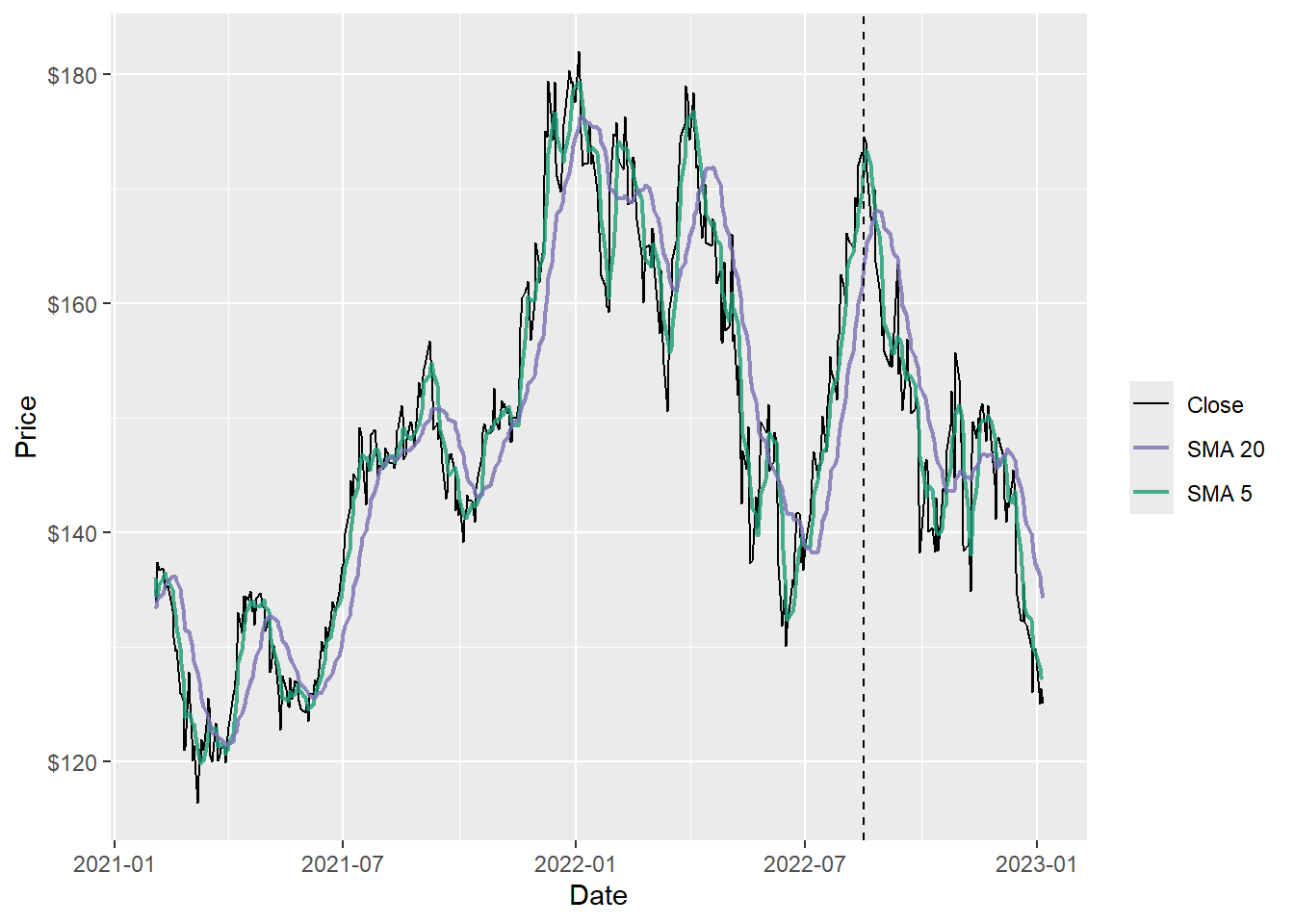
The short moving average follows the closing price more closely than the long moving average. When the short and long averages separate or cross, they summarize recent momentum changes. These signals are useful as inputs, but they remain noisy because price reversals can happen quickly.
The final observations make the timing difference clearer.
Code
tail(trading_tbl, 30) %>%
  ggplot(aes(date)) +
  geom_line(aes(y = close, color = "Close"), linewidth = 0.7) +
  geom_line(aes(y = sma_5, color = "SMA 5"), linewidth = 2.5, alpha = 0.6) +
  geom_line(aes(y = sma_20, color = "SMA 20"), linewidth = 2.5, alpha = 0.6) +
  scale_color_manual(values = c("Close" = "black",
                                "SMA 5" = "#1B9E77",
                                "SMA 20" = "#7570B3")) +
  labs(x = "Date", y = "Price", color = "") +
  scale_y_continuous(labels = scales::dollar)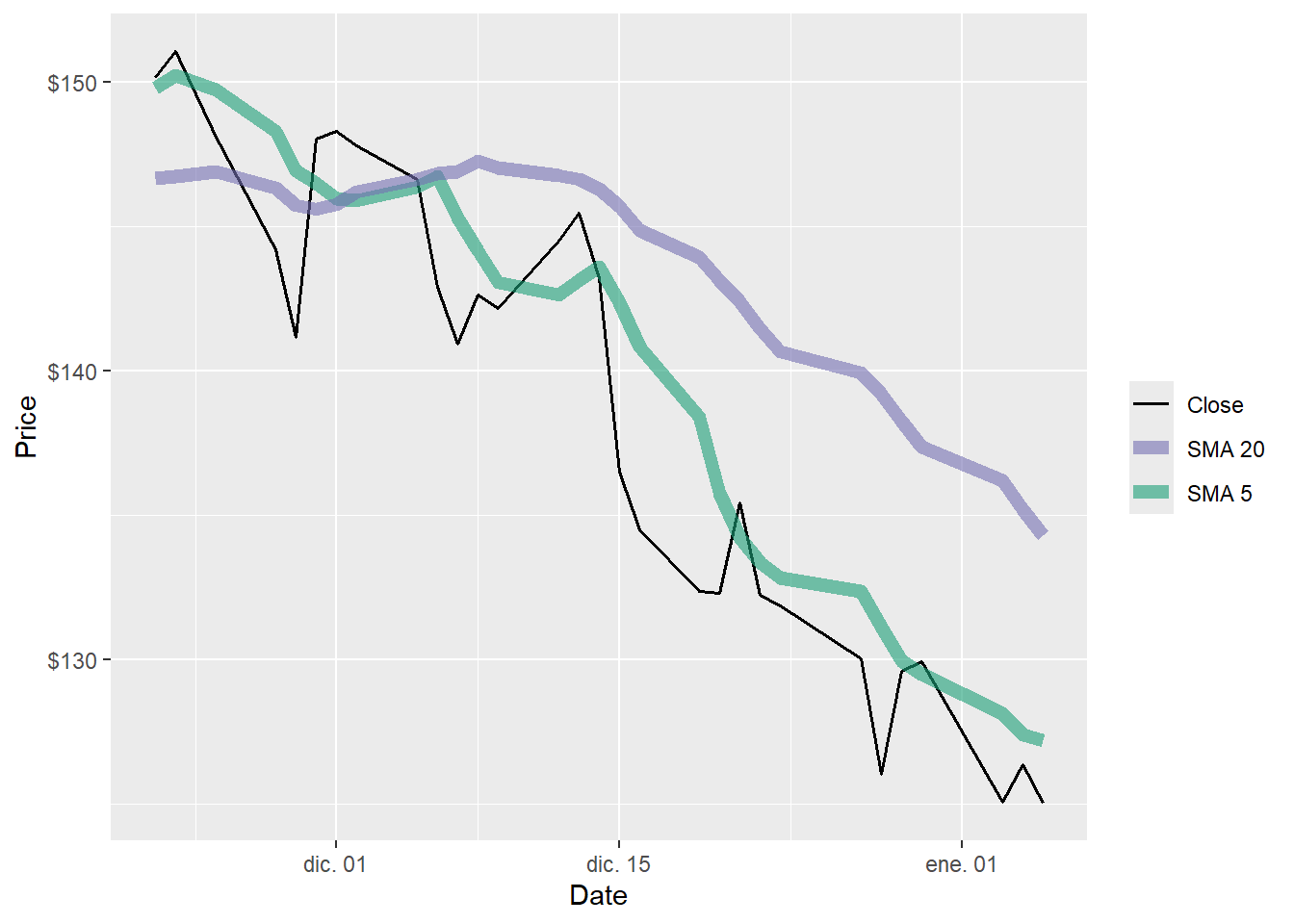
The zoom makes the timing problem visible. The 5-day average reacts first, while the 20-day average moves more slowly. The classifier uses lagged versions of these curves, so the trading decision is based on information available before the return being evaluated.
3.4 Preliminaries to classify returns
The modeling objective is to anticipate positive and negative daily stock price movements. The response variable has two classes.
Upmeans the realized daily return was positive;Downmeans the realized daily return was zero or negative.
The lagged moving averages are the predictor variables \(X\), and the current return direction is the target variable \(y\).
This gives the following classification table.
\[ \left(x_{t-1}, d_t\right) = \left( \text{SMA}_{5,t-1}, \text{SMA}_{10,t-1}, \text{SMA}_{15,t-1}, \text{SMA}_{20,t-1}, d_t \right). \]
The timing is now explicit. The features in row \(t\) are moving averages known at the end of day \(t-1\), while the label is the return direction realized over day \(t\). The trading decision is therefore based on yesterday’s information.
Code
model_tbl <- trading_tbl %>%
  mutate(direction = factor(if_else(return > 0, "Up", "Down"),
                            levels = c("Down", "Up")),
         sma_5_lag1 = dplyr::lag(sma_5),
         sma_10_lag1 = dplyr::lag(sma_10),
         sma_15_lag1 = dplyr::lag(sma_15),
         sma_20_lag1 = dplyr::lag(sma_20)) %>%
  filter(complete.cases(.)) %>%
  select(date, close, return, sma_5_lag1, sma_10_lag1, sma_15_lag1,
         sma_20_lag1, direction)

head(model_tbl)
# A tibble: 6 × 8
date close return sma_5_lag1 sma_10_lag1 sma_15_lag1 sma_20_lag1
<date> <dbl> <dbl> <dbl> <dbl> <dbl> <dbl>
1 2021-02-03 134. -0.00778 136. 137. 135. 133.
2 2021-02-04 137. 0.0258 134. 138. 135. 134.
3 2021-02-05 137. -0.00459 134. 138. 135. 134.
4 2021-02-08 137. 0.00110 135. 137. 136. 134.
5 2021-02-09 136. -0.00657 136. 137. 136. 135.
6 2021-02-10 135. -0.00456 136. 136. 137. 135.
# ℹ 1 more variable: direction <fct>Both training and test sets are split in time order. The data are not shuffled because that would mix past and future observations.
The training set is the first 80% of the observations and the test set is the remaining 20%.
\[ \mathcal{T}_{train} = \{1,\ldots,T_0\}, \qquad \mathcal{T}_{test} = \{T_0+1,\ldots,T\}. \]
The model is fitted only on \(\mathcal{T}_{train}\). The test set is reserved for classification and trading evaluation.
Code
split_index <- floor(nrow(model_tbl) * 0.8)

train_tbl <- model_tbl[seq_len(split_index), ]
test_tbl <- model_tbl[(split_index + 1):nrow(model_tbl), ]
split_date <- min(test_tbl$date)

tibble(
  sample = c("Train", "Test"),
  observations = c(nrow(train_tbl), nrow(test_tbl)),
  start = c(min(train_tbl$date), min(test_tbl$date)),
  end = c(max(train_tbl$date), max(test_tbl$date))
) %>%
  kable(caption = "Time-ordered train/test split.") %>%
kable_styling(latex_options = "HOLD_position")| sample | observations | start | end |
|---|---|---|---|
| Train | 388 | 2021-02-03 | 2022-08-17 |
| Test | 97 | 2022-08-18 | 2023-01-05 |
3.5 Set up the model
A random forest is estimated. A random forest is an ensemble of decision trees. Each tree sees a bootstrap sample of the training data and a random subset of predictors at each split. The final class is chosen by majority vote.
If the forest has \(B\) trees, each tree votes for either Up or Down. The vote counts for both classes are defined below.
\[ V_{\text{Up}} = \text{number of trees voting Up}, \qquad V_{\text{Down}} = \text{number of trees voting Down}. \]
The predicted direction is simply the class with more votes.
In the code below, \(B=500\) and mtry = 2. The first choice means the forest combines 500 trees, which reduces the noise of relying on one single tree. The second choice means each split considers two of the four lagged moving-average predictors. These are fixed modeling choices for this teaching example. They are not selected to maximize the test return.
Code
Call:
 randomForest(formula = direction ~ sma_5_lag1 + sma_10_lag1 +      sma_15_lag1 + sma_20_lag1, data = train_tbl, ntree = 500,      mtry = 2, nodesize = 1)
               Type of random forest: classification
                     Number of trees: 500
No. of variables tried at each split: 2

        OOB estimate of  error rate: 51.8%
Confusion matrix:
     Down Up class.error
Down   90 98   0.5212766
Up    103 97   0.5150000
3.6 Evaluate the model
The following helper function calculates classification accuracy and a confusion matrix. Predictions are created from the vote counts with an explicit tie rule. If the vote is exactly tied, the helper returns Down. That rule keeps the backtest reproducible.
The implemented rule is therefore
\[ \hat{g}(x_{t-1}) = \begin{cases} \text{Up}, & V_{\text{Up}}(x_{t-1}) > V_{\text{Down}}(x_{t-1}),\\ \text{Down}, & V_{\text{Up}}(x_{t-1}) \leq V_{\text{Down}}(x_{t-1}). \end{cases} \]
Classification accuracy is the proportion of days classified correctly.
\[ \text{Accuracy} = \frac{\text{number of correct predictions}}{\text{number of predictions}}. \]
Code
predict_direction <- function(fit, new_data) {
  votes <- predict(fit, newdata = new_data, type = "vote", norm.votes = FALSE)
  factor(
    if_else(votes[, "Up"] > votes[, "Down"], "Up", "Down"),
    levels = levels(train_tbl$direction)
  )
}

accuracy_value <- function(actual, predicted) {
  mean(actual == predicted)
}
Training performance is evaluated first.
Code
| Down | Up | |
|---|---|---|
| Down | 188 | 0 |
| Up | 0 | 200 |
[1] 1Test performance is evaluated next.
Code
| Down | Up | |
|---|---|---|
| Down | 30 | 26 |
| Up | 14 | 27 |
[1] 0.5876289This result should be interpreted carefully. Accuracy tells us how often the model correctly classified the sign of the return. It does not tell us whether the trading strategy makes money. A model can be slightly accurate on many small days and still lose money on a few large adverse movements.
Code
tibble(
  sample = c("Train", "Test"),
  accuracy = c(
    accuracy_value(train_tbl$direction, pred_train),
    accuracy_value(test_tbl$direction, pred_test)
  ),
  positive_days = c(sum(train_tbl$direction == "Up"),
                    sum(test_tbl$direction == "Up")),
  negative_days = c(sum(train_tbl$direction == "Down"),
                    sum(test_tbl$direction == "Down"))
) %>%
  kable(caption = "Directional classification summary.", digits = 3) %>%
kable_styling(latex_options = "HOLD_position")| sample | accuracy | positive_days | negative_days |
|---|---|---|---|
| Train | 1.000 | 200 | 188 |
| Test | 0.588 | 41 | 56 |
3.7 Trading rules and backtest
The predicted class is translated into three trading rules. Since the prediction uses lagged moving averages, the position for day \(t\) is based on information available before \(r_t\) is realized.
The conservative long/cash rule is
\[ q_t = \begin{cases} 1, & \text{if the model predicts Up},\\ 0, & \text{if the model predicts Down}. \end{cases} \]
\[ R_t^{LC} = q_t r_t. \]
This rule answers a conservative allocation question about market exposure. It never shorts the stock. When the model predicts Down, the strategy avoids exposure to the decline.
The aggressive long/short rule is
\[ R_t^{LS} = p_t r_t, \qquad p_t = \begin{cases} 1, & \text{if the model predicts Up},\\ -1, & \text{if the model predicts Down}. \end{cases} \]
This rule answers a stronger directional question about long versus short exposure. It is always exposed to the stock. A correct Down prediction can make money because the short position gains when the stock return is negative. The trade-off is that a wrong Down prediction loses money when the stock rises, and short positions introduce operational constraints that cash positions do not have.
The third rule applies trading and short-selling costs to the long/short rule.
\[ R_t^{LS,net} = p_t r_t - c_{trade}|p_t-p_{t-1}| - c_{short}\mathbf{1}(p_t=-1). \]
So the short cost is charged only on days when the strategy is short. If \(p_t=1\), that last cost term is zero.
This rule tests whether the long/short result survives basic trading frictions. It uses the same signal as the gross long/short rule, with returns reduced when the strategy changes position and when it holds a short position.
At the beginning of the test period, the strategy starts from cash. Therefore, entering the first long or short position counts as a position change and pays the corresponding trading friction. This keeps the comparison anchored to the same initial capital for all strategies.
Code
rule_map <- tibble(
  `Rule` = c("Long/cash", "Long/short gross", "Long/short net of costs"),
  `If prediction is<br>Up` = c("+1 long", "+1 long", "+1 long"),
  `If prediction is<br>Down` = c("0 cash", "-1 short", "-1 short"),
  `Return<br>rule` = c(
    "\\(R_t^{LC} = q_t r_t\\)",
    "\\(R_t^{LS} = p_t r_t\\)",
    paste0(
      "\\(R_t^{LS,net} = p_t r_t - c_{trade}",
      "\\lvert p_t - p_{t-1}\\rvert - ",
      "c_{short}\\text{ if }p_t=-1\\)"
    )
  ),
  `Reading` = c(
    "Conservative timing rule: participate only when the model expects an up day.",
    "Aggressive directional rule: be long on expected up days and short on expected down days.",
    "Same long/short exposure, but reduced by trading frictions and short-borrow cost."
  )
)

kable(rule_map,
      format = "html",
      caption = "Economic reading of the three robo trader rules.",
      escape = FALSE,
      row.names = FALSE) %>%
kable_styling(latex_options = "HOLD_position")| Rule | If prediction is Up |
If prediction is Down |
Return rule |
Reading |
|---|---|---|---|---|
| Long/cash | +1 long | 0 cash | \(R_t^{LC} = q_t r_t\) | Conservative timing rule: participate only when the model expects an up day. |
| Long/short gross | +1 long | -1 short | \(R_t^{LS} = p_t r_t\) | Aggressive directional rule: be long on expected up days and short on expected down days. |
| Long/short net of costs | +1 long | -1 short | \(R_t^{LS,net} = p_t r_t - c_{trade}\lvert p_t - p_{t-1}\rvert - c_{short}\text{ if }p_t=-1\) | Same long/short exposure, but reduced by trading frictions and short-borrow cost. |
Here, \(c_{trade}\) captures trading frictions such as commissions, bid-ask spread and slippage, while \(c_{short}\) captures the daily cost of borrowing shares for short exposure. The base scenario uses 5 basis points per unit of position change and 1 basis point per short day, approximately 2.52% annualized over 252 trading days. These are pedagogical assumptions, not broker-specific quotes.
The cost assumptions are not meant to be exact current costs for AAPL at one specific broker. They are a transparent backtest haircut. The commission part can be low for U.S. stocks at some brokers; for example, Interactive Brokers lists zero-commission U.S. stocks and ETFs for IBKR Lite and low per-share commissions for IBKR Pro (Interactive Brokers commissions). Explicit commissions are only one part of trading cost. A backtest also needs to reserve room for bid-ask spread and slippage. For the short leg, Interactive Brokers documents that short-sale cost depends on the borrow fee, collateral value and daily accrual (Interactive Brokers short sale cost). Short selling also requires borrow and delivery mechanics under Regulation SHO (SEC Regulation SHO) and is tied to margin requirements (FINRA margin accounts).
Code
cost_assumptions <- tibble(
  cost_component = c("Trading friction", "Short-borrow cost"),
  parameter = c("trade_cost", "short_cost_daily"),
  value = c("0.0005", "0.0001"),
  basis_points = c("5 bps", "1 bp"),
  applied_when = c(
    "Every unit of long/short position change",
    "Every day the long/short rule is short"
  ),
  reading = c(
    "Commission, bid-ask spread and slippage haircut.",
    "Daily stock-borrow cost; 1 bp per day is about 2.52% per year."
  )
)

kable(cost_assumptions,
      caption = "Base cost assumptions for the net long/short rule.",
      row.names = FALSE) %>%
kable_styling(latex_options = "HOLD_position")| cost_component | parameter | value | basis_points | applied_when | reading |
|---|---|---|---|---|---|
| Trading friction | trade_cost | 0.0005 | 5 bps | Every unit of long/short position change | Commission, bid-ask spread and slippage haircut. |
| Short-borrow cost | short_cost_daily | 0.0001 | 1 bp | Every day the long/short rule is short | Daily stock-borrow cost; 1 bp per day is about 2.52% per year. |
For every rule, cumulative value is computed as
\[ C_t = \prod_{i=1}^{t}(1+R_i). \]
Code
trade_cost <- 0.0005
short_cost_daily <- 0.0001

all_predictions <- model_tbl %>%
  mutate(
    predicted_direction = predict_direction(fit_rf, model_tbl),
    long_cash_position = if_else(predicted_direction == "Up", 1, 0),
    long_short_position = if_else(predicted_direction == "Up", 1, -1),
    long_cash_return = long_cash_position * return,
    long_short_return = long_short_position * return,
    buy_hold_return = return
  )

test_strategy <- all_predictions %>%
  filter(date >= split_date) %>%
  mutate(
    long_cash_signal = long_cash_position -
      dplyr::lag(long_cash_position, default = 0),
    long_short_position_change = abs(
      long_short_position - dplyr::lag(long_short_position, default = 0)
    ),
    long_short_net_return = long_short_return -
      trade_cost * long_short_position_change -
      short_cost_daily * as.numeric(long_short_position == -1),
    cumulative_long_cash = cumprod(1 + long_cash_return),
    cumulative_long_short = cumprod(1 + long_short_return),
    cumulative_long_short_net = cumprod(1 + long_short_net_return),
    cumulative_buy_hold = cumprod(1 + buy_hold_return)
  )

test_strategy %>%
  transmute(
    `Date` = date,
    `Return<br>r_t` = return,
    `Predicted<br>direction` = predicted_direction,
    `LC<br>position` = long_cash_position,
    `LS<br>position` = long_short_position,
    `LC<br>return` = long_cash_return,
    `LS gross<br>return` = long_short_return,
    `LS net<br>return` = long_short_net_return,
    `LC<br>value` = cumulative_long_cash,
    `LS net<br>value` = cumulative_long_short_net
  ) %>%
  head(10) %>%
  kable(format = "html",
        caption = "First test observations for the trading rules.",
        digits = 4,
        escape = FALSE) %>%
  add_header_above(c("Date and signal" = 3,
                     "Positions" = 2,
                     "Daily returns" = 3,
                     "Cumulative value" = 2),
                   escape = FALSE) %>%
kable_styling(latex_options = "HOLD_position")| Date | Return r_t |
Predicted direction |
LC position |
LS position |
LC return |
LS gross return |
LS net return |
LC value |
LS net value |
|---|---|---|---|---|---|---|---|---|---|
| 2022-08-18 | -0.0023 | Up | 1 | 1 | -0.0023 | -0.0023 | -0.0028 | 0.9977 | 0.9972 |
| 2022-08-19 | -0.0151 | Up | 1 | 1 | -0.0151 | -0.0151 | -0.0151 | 0.9826 | 0.9821 |
| 2022-08-22 | -0.0230 | Up | 1 | 1 | -0.0230 | -0.0230 | -0.0230 | 0.9600 | 0.9595 |
| 2022-08-23 | -0.0020 | Down | 0 | -1 | 0.0000 | 0.0020 | 0.0009 | 0.9600 | 0.9604 |
| 2022-08-24 | 0.0018 | Down | 0 | -1 | 0.0000 | -0.0018 | -0.0019 | 0.9600 | 0.9586 |
| 2022-08-25 | 0.0149 | Down | 0 | -1 | 0.0000 | -0.0149 | -0.0150 | 0.9600 | 0.9442 |
| 2022-08-26 | -0.0377 | Down | 0 | -1 | 0.0000 | 0.0377 | 0.0376 | 0.9600 | 0.9797 |
| 2022-08-29 | -0.0137 | Up | 1 | 1 | -0.0137 | -0.0137 | -0.0147 | 0.9469 | 0.9653 |
| 2022-08-30 | -0.0153 | Up | 1 | 1 | -0.0153 | -0.0153 | -0.0153 | 0.9324 | 0.9505 |
| 2022-08-31 | -0.0106 | Down | 0 | -1 | 0.0000 | 0.0106 | 0.0095 | 0.9324 | 0.9596 |
This is the final return comparison over the test period. For a strategy return series \(r^s_1,\ldots,r^s_T\), the final value and total return are defined below.
\[ F_T=\prod_{t=1}^{T}(1+r^s_t), \qquad TR=F_T-1. \]
Code
strategy_summary <- tibble(
  strategy = c(
    "Robo trader: long/cash",
    "Robo trader: long/short gross",
    "Robo trader: long/short net of costs",
    "Buy and hold"
  ),
  final_value = c(
    tail(test_strategy$cumulative_long_cash, 1),
    tail(test_strategy$cumulative_long_short, 1),
    tail(test_strategy$cumulative_long_short_net, 1),
    tail(test_strategy$cumulative_buy_hold, 1)
  )
) %>%
  mutate(total_return = final_value - 1)

strategy_summary %>%
  mutate(total_return = scales::percent(total_return, accuracy = 0.01)) %>%
  rename("Strategy" = strategy,
         "Final Value" = final_value,
         "Total Return" = total_return) %>%
  kable(caption = "Final cumulative return comparison.",
        digits = 4) %>%
kable_styling(latex_options = "HOLD_position")| Strategy | Final Value | Total Return |
|---|---|---|
| Robo trader: long/cash | 1.0338 | 3.38% |
| Robo trader: long/short gross | 1.4673 | 46.73% |
| Robo trader: long/short net of costs | 1.4185 | 41.85% |
| Buy and hold | 0.7162 | -28.38% |
The net result uses the base cost assumptions above. To check whether that conclusion depends too much on one cost number, three cost scenarios are evaluated. The signal and the positions are unchanged; only the cost haircut changes. The net daily return is defined below.
\[ r^{net}_t = r^{long/short}_t - c^{trade}\Delta position_t - c^{short}\mathbf{1}(position_t=-1). \]
Code
cost_scenarios <- tibble(
  scenario = c("Low cost", "Base cost", "High cost"),
  trade_cost = c(0.0001, 0.0005, 0.0010),
  short_cost_daily = c(0.00002, 0.00010, 0.00020)
)

cost_sensitivity <- cost_scenarios %>%
  rowwise() %>%
  mutate(
    annual_short_cost = short_cost_daily * 252,
    final_value = {
      net_return <- test_strategy$long_short_return -
        trade_cost * test_strategy$long_short_position_change -
        short_cost_daily * as.numeric(test_strategy$long_short_position == -1)
      tail(cumprod(1 + net_return), 1)
    },
    total_return = final_value - 1
  ) %>%
  ungroup()

cost_sensitivity %>%
  mutate(
    trade_cost_bps = trade_cost * 10000,
    short_cost_daily_bps = short_cost_daily * 10000,
    annual_short_cost = scales::percent(annual_short_cost, accuracy = 0.01),
    total_return = scales::percent(total_return, accuracy = 0.01)
  ) %>%
  select(scenario, trade_cost_bps, short_cost_daily_bps,
         annual_short_cost, final_value, total_return) %>%
  rename("Scenario" = scenario,
         "Trade Cost (bps)" = trade_cost_bps,
         "Daily Short Cost (bps)" = short_cost_daily_bps,
         "Annual Short Cost" = annual_short_cost,
         "Final Value" = final_value,
         "Total Return" = total_return) %>%
  kable(caption = "Cost sensitivity for the long/short rule.",
        digits = 4,
        row.names = FALSE) %>%
kable_styling(latex_options = "HOLD_position")| Scenario | Trade Cost (bps) | Daily Short Cost (bps) | Annual Short Cost | Final Value | Total Return |
|---|---|---|---|---|---|
| Low cost | 1 | 0.2 | 0.50% | 1.4574 | 45.74% |
| Base cost | 5 | 1.0 | 2.52% | 1.4185 | 41.85% |
| High cost | 10 | 2.0 | 5.04% | 1.3714 | 37.14% |
The sensitivity table is a first robustness check. It asks whether the long/short result remains visible after basic costs are included. A more serious trading study would test many assets, many periods and broker-specific cost assumptions.
The long/cash rule is the most conservative reading of the classifier because a Down prediction simply removes market exposure. The long/short rule is more powerful in a falling market because a Down prediction becomes a short position. This explains why its gross cumulative return is much higher in this test window: Apple declined substantially, and the model predicted Down on 44 of the 97 test days. On those days, long/cash has zero exposure, while long/short tries to earn the opposite of the stock return. The net long/short rule keeps the same directional exposure but asks whether the advantage is large enough to remain after trading frictions and short-borrow costs.
The comparison uses the same classifier in all three robo trader rules. Only the portfolio mapping changes.
\[ \hat{g}(x_{t-1}) \longrightarrow \text{position} \longrightarrow \text{strategy return}. \]
That is useful pedagogically because it separates the machine-learning task from the trading-design task. The classifier produces directional information, and the trading rule converts that information into exposure.
The following table summarizes how often the strategy is invested and how often it moves between positions.
Code
test_strategy %>%
  summarise(
    `Test days` = n(),
    `Long/cash invested days` = sum(long_cash_position == 1),
    `Long/cash cash days` = sum(long_cash_position == 0),
    `Long/short long days` = sum(long_short_position == 1),
    `Long/short short days` = sum(long_short_position == -1),
    `Long/short switches` = sum(long_short_position_change > 0),
    `Total position change` = sum(long_short_position_change)
  ) %>%
  tidyr::pivot_longer(
    cols = everything(),
    names_to = "Measure",
    values_to = "Value"
  ) %>%
  kable(caption = "Trading activity during the test period.",
        digits = 0) %>%
kable_styling(latex_options = "HOLD_position")| Measure | Value |
|---|---|
| Test days | 97 |
| Long/cash invested days | 53 |
| Long/cash cash days | 44 |
| Long/short long days | 53 |
| Long/short short days | 44 |
| Long/short switches | 30 |
| Total position change | 59 |
The long/cash rule has cash days because it refuses exposure after a Down prediction. The long/short rule has no cash days by design: every day is either long or short. The number of long/short switches matters because trading costs are charged when the desired position changes. A move from long to short is a two-unit change in exposure, from \(+1\) to \(-1\), so it is more expensive than moving from cash to long.
The cumulative comparison places the robo trader rules against buy-and-hold over the test period.
Code
strategy_long <- bind_rows(
  test_strategy %>%
    transmute(date, strategy = "Long/cash", value = cumulative_long_cash),
  test_strategy %>%
    transmute(date, strategy = "Long/short gross",
              value = cumulative_long_short),
  test_strategy %>%
    transmute(date, strategy = "Long/short net of costs",
              value = cumulative_long_short_net),
  test_strategy %>%
    transmute(date, strategy = "Buy and hold", value = cumulative_buy_hold)
)

strategy_long %>%
  ggplot(aes(date, value, color = strategy)) +
  geom_line(linewidth = 0.8) +
  scale_color_manual(values = c(
    "Long/cash" = "#1B9E77",
    "Long/short gross" = "#7570B3",
    "Long/short net of costs" = "#D95F02",
    "Buy and hold" = "black"
  )) +
  labs(x = "Date", y = "Cumulative return", color = "")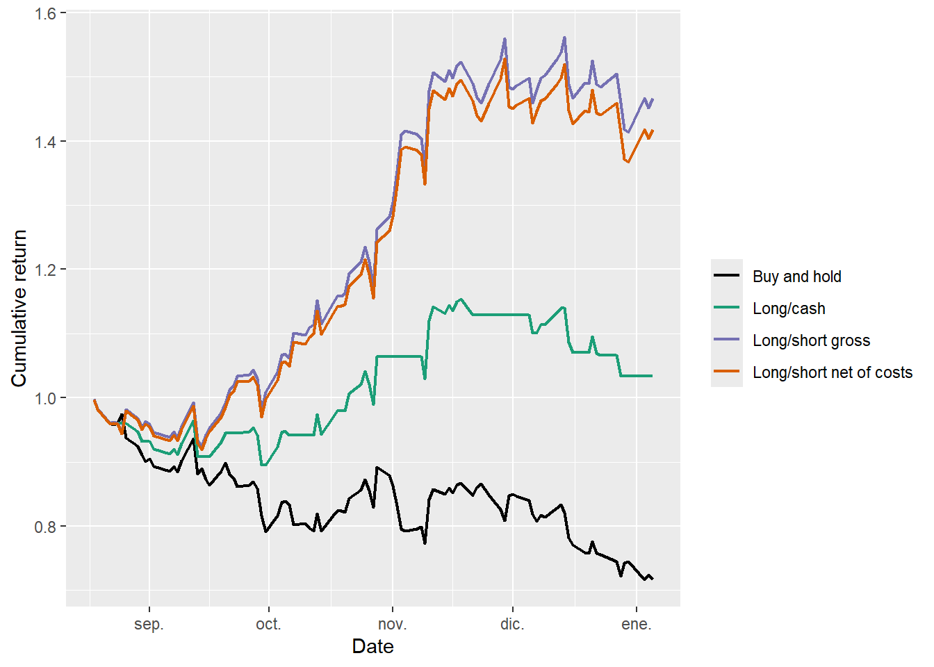
The buy-and-hold line declines through the test window. The long/cash rule is more defensive because it can step out of the market after a Down prediction. The long/short rule performs best in this historical window because many Down predictions coincide with negative AAPL returns. Costs reduce the long/short value, which is why the net line is below the gross line. The figure therefore separates three ideas: prediction, position choice, and implementation cost.
The conclusion is deliberately narrow. The chapter shows how to translate a classification model into a trading rule and how to compute the resulting cumulative return under a clear timing convention. The net long/short rule also shows how sensitive the result is to explicit trading frictions. Establishing a profitable trading strategy would require broader cost sensitivity, position limits, risk measures, drawdowns, alternative train/test splits and live out-of-sample monitoring.
The next chapter changes the question from short-run direction to systematic return exposure. After asking whether a rule predicts tomorrow’s up or down movement, the next question asks how much of an asset’s return can be associated with market movements and other risk factors. That shift takes the book from trading signals to return co-movement and beta.