The previous chapters worked with market data, returns, trading rules, asset pricing, portfolio allocation, and market risk. This chapter changes the object of analysis. A blockchain is treated here as a financial-computing mechanism: a way to maintain a shared record of transfers, validate changes to that record, and coordinate incentives without requiring a single central ledger.
The financial question is direct: how can a system record transfers of value when many participants can read the ledger, submit transactions, and verify the history? The answer combines several ideas:
a ledger that records transactions;
blocks that group transactions;
cryptographic hashes that link blocks;
digital signatures that authorize transactions;
a consensus rule that tells nodes which history to accept;
incentives that reward participants who help maintain the ledger.
The chapter uses Bitcoin as the motivating case, then builds the technical pieces needed to understand it. Bitcoin is useful because it turns a ledger mechanism into an economic system with wallets, private keys, miners, fees, scarce issuance, public verification, and costly history rewriting. Once those pieces are visible, tokenization becomes a natural financial extension: a ledger can also record ownership units and cash-flow allocation rules for claims whose value may depend on assets outside the ledger.
The examples are intentionally small teaching models. They show the logic of the system at a scale where each moving part can be inspected.
A useful way to read the chapter is through four frictions: a user may try to spend the same value twice; block space can become scarce; settlement becomes more reliable as confirmations accumulate; tokenized claims need a connection between the ledger record and the legal or operational asset. These frictions make blockchain a financial topic, because they connect technology to scarcity, incentives, custody, and settlement.
7.1 Bitcoin as motivating case
Students usually meet blockchain through Bitcoin prices, wallets, exchanges, and transaction confirmations. Those entry points are useful, but they hide the mechanism. A Bitcoin payment is a signed instruction that spends previous outputs, moves through a peer-to-peer network, competes for block space, and becomes harder to reverse as proof-of-work accumulates above it.
The financial modeling question is therefore richer than “what is the price of Bitcoin?” We also need to ask:
Object
Modeling question
Financial meaning
Private key
Who can authorize spending?
Custody and operational control
Transaction
Which value is being transferred, and under what fee?
Payment, settlement, and fee pressure
Block
Which transactions enter the next ledger update?
Scarce inclusion and audit trail
Proof-of-work
How costly is it to replace recent history?
Settlement confidence
Network
How do transactions and blocks propagate?
Latency, monitoring, and public observability
Token rule
What claim does a ledger entry represent?
Ownership, cash-flow allocation, and legal linkage
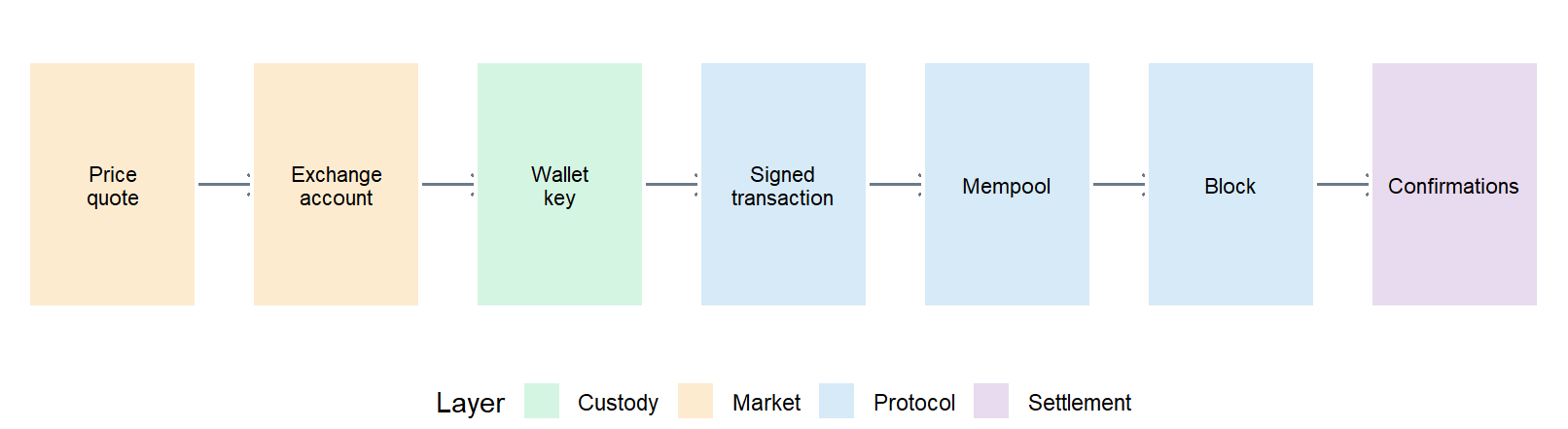
The path from familiar market objects to protocol mechanics can be drawn as a short workflow.
Figure 7.1: From market-facing Bitcoin objects to protocol mechanics.
The figure sets the chapter’s stance. A price quote or an exchange account is one visible surface of the system. The modeling work begins when custody, authorization, pending settlement, block inclusion, and confirmations are tied to the same record of value.
The rest of the chapter builds these objects in small pieces. Each teaching model corresponds to a production concern: double spending, block construction, signatures, custody, network propagation, confirmations, and tokenized claims.
7.2 Generic blockchain model
The generic model is a compact laboratory for the Bitcoin case. It uses an account-based ledger because balances are easy to read: each wallet has a balance, transactions move value across wallets, fees compensate the block producer, and the final ledger state can be checked directly. Bitcoin uses a different accounting model, based on unspent transaction outputs, and that difference is introduced after the generic mechanism is in place.
The generic model answers four questions:
Component
Question
Financial role
Ledger state
Who owns what before and after transfers?
Records balances or ownership claims
Transaction rule
Which transfers are valid?
Prevents invalid spending and malformed transfers
Block structure
Which transactions enter the next ledger update?
Groups accepted transfers into an auditable batch
Consensus rule
Which history should nodes extend?
Coordinates participants around one accepted ledger
A conventional financial ledger records who owns what and how balances change after transactions. In a centralized system, one institution updates the ledger, rejects invalid transfers, and resolves conflicts. A blockchain moves part of that logic into a shared protocol: many participants can hold copies of the ledger, check the same rules, and converge on an accepted history.
The most basic financial state is a table of balances. Suppose four wallets start with the following balances.
This accounting rule is the starting point for the blockchain workflow. The ledger state gives balances at one moment; the block history explains how those balances were reached. For finance, that audit path matters because ownership claims are stronger when they can be traced through accepted transactions.
Double-spending pressure
The first interesting problem is conflict. If Alice has 100 units and submits two transactions that each spend about 70 units, both transactions cannot settle inside the same ledger history:
\[
x_1+f_1+x_2+f_2 > \mathrm{Balance}_A.
\]
The system needs a rule for deciding which transaction enters the accepted history. In a centralized ledger the institution decides. In a blockchain network, the accepted history comes from transaction validity, block inclusion, and consensus.
# A tibble: 4 × 8
  tx_id sender receiver amount   fee total_spent status   ordering
  <chr> <chr>  <chr>     <dbl> <dbl>       <dbl> <chr>    <chr>
1 tx_A  Alice  Bob          70   0.2        70.2 Accepted tx_A arrives first
2 tx_B  Alice  Carol        70   0.4        70.4 Rejected tx_A arrives first
3 tx_B  Alice  Carol        70   0.4        70.4 Accepted Higher fee arrives fi…
4 tx_A  Alice  Bob          70   0.2        70.2 Rejected Higher fee arrives fi…
Code
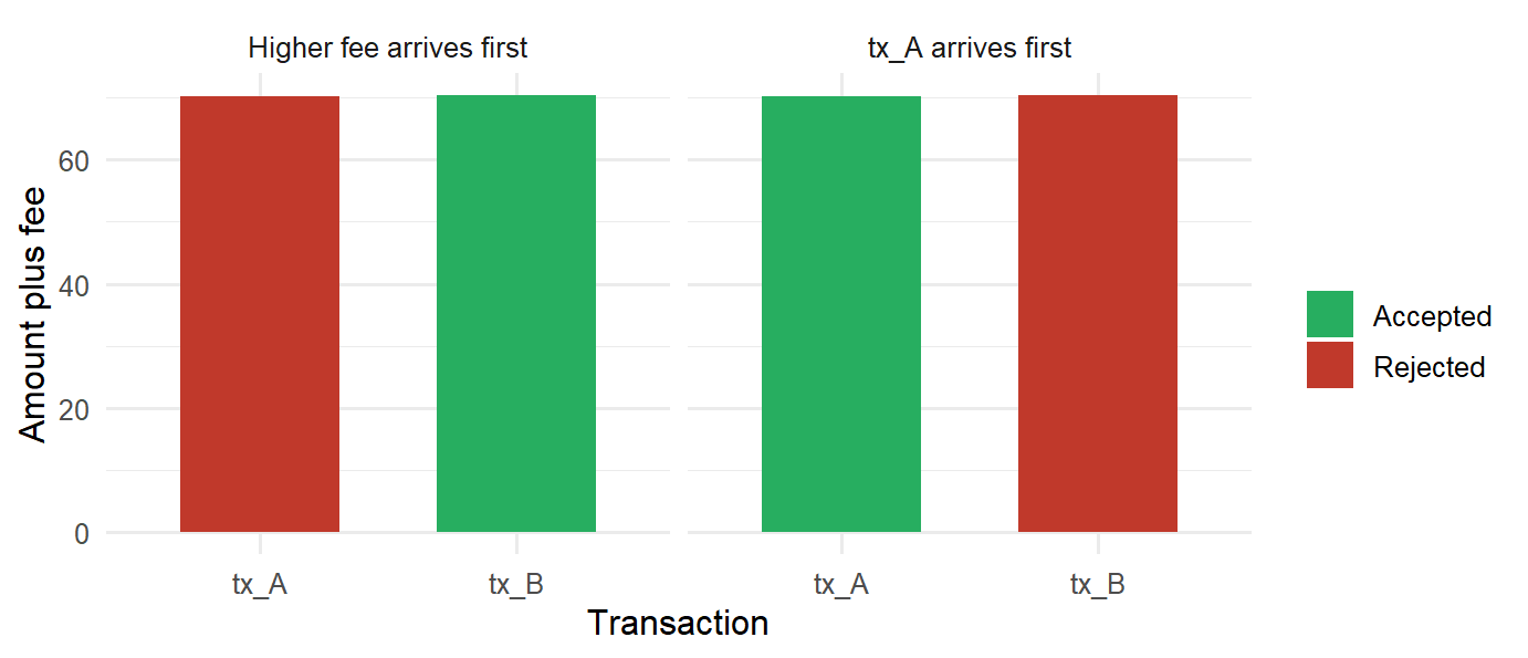
ggplot( double_spend_outcome,aes(x = tx_id, y = total_spent, fill = status)) +geom_col(width =0.62) +facet_wrap(~ ordering) +scale_fill_manual(values =c("Accepted"="#27AE60","Rejected"="#C0392B")) +labs(x ="Transaction", y ="Amount plus fee", fill ="")
Figure 7.2: Conflicting transactions under two ordering rules.
The figure shows why a shared ledger needs more than arithmetic. The balances tell us that the two transfers cannot both be final. The network still needs a mechanism for selecting one accepted history and rejecting conflicting updates.
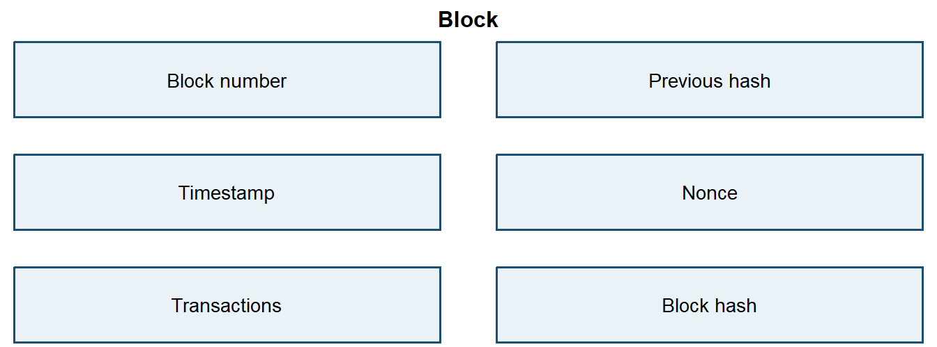
Blocks
A block is a container for ledger information. In a simple teaching example, the block contains:
block <-list(number =1,timestamp ="2026-01-01 09:00:00",data ="Alice pays Bob 10",parent_hash ="0",nonce =0)tibble(field =names(block),value =vapply(block, as.character, character(1)))
# A tibble: 5 × 2
  field       value
  <chr>       <chr>
1 number      1
2 timestamp   2026-01-01 09:00:00
3 data        Alice pays Bob 10
4 parent_hash 0
5 nonce       0
This object still needs a hash before it can be chained to a history.
The block gives the system a unit of agreement. The network evaluates a batch of transactions together with the previous history that the batch extends. The parent hash records that link: it identifies the past ledger state that the new block is trying to update.
Hashes
A cryptographic hash function maps an input of arbitrary size into a fixed-size digest. A useful hash function for a ledger has three properties:
the same input gives the same hash;
a small change in the input gives a very different hash;
the input cannot be reconstructed from the hash in any practical way.
For non-genesis blocks, the parent hash equals the hash of the previous block:
\[
\mathrm{parentHash}_i = h_{i-1}.
\]
The examples use SHA-256 through the digest package. SHA-256 returns 256 bits, which correspond to 32 bytes or 64 hexadecimal characters.
Code
hash_example <-digest("Alice pays Bob 10", algo ="sha256")tibble(message ="Alice pays Bob 10",algorithm ="SHA-256",hex_characters =nchar(hash_example),hash_prefix =substr(hash_example, 1, 16))
# A tibble: 1 × 4
  message           algorithm hex_characters hash_prefix
  <chr>             <chr>              <int> <chr>
1 Alice pays Bob 10 SHA-256               64 70e9b38977e6fb5a
A tiny change in the message changes the digest.
Code
hash_comparison <-tibble(message =c("Alice pays Bob 10", "Alice pays Bob 11"),sha256 =vapply(message, digest, character(1), algo ="sha256")) |>mutate(hash_prefix =substr(sha256, 1, 18)) |>select(message, hash_prefix)hash_comparison
# A tibble: 2 × 2
  message           hash_prefix
  <chr>             <chr>
1 Alice pays Bob 10 70e9b38977e6fb5acc
2 Alice pays Bob 11 d8e09925fe69f7daf2
The table shows only hash prefixes to keep the output readable. The important point is that the two prefixes already diverge after a one-character change, while each full SHA-256 digest remains 64 hexadecimal characters long.
The following helper creates a block and then hashes the full block content.
# A tibble: 3 × 4
  block data              parent_hash  block_hash
  <dbl> <chr>             <chr>        <chr>
1     1 Genesis block     0            884045791d17
2     2 Alice pays Bob 10 884045791d17 d6ab66a54c32
3     3 Bob pays Carol 5  d6ab66a54c32 3db2457c9284
The summary keeps the block order, data, parent commitment, and block commitment visible without printing the full nested R objects.
The financial meaning of this construction is integrity. A block hash is a compact cryptographic commitment to the block content, and a parent hash is a commitment to the previous accepted history. Linking those commitments means that the latest block implicitly refers to every earlier accepted block. If an old transaction changes, the old hash changes, and later blocks no longer point to the same history.
Chain validation
A basic validation rule checks two conditions:
each block hash matches the content of that block;
each non-genesis block points to the hash of the previous block.
# A tibble: 1 × 2
  check          valid
  <chr>          <lgl>
1 Original chain TRUE
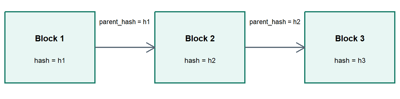
The chain can be drawn as a sequence of blocks connected by hashes.
Code
chain_plot <-tibble(block =c("Block 1", "Block 2", "Block 3"),x =c(1, 4, 7),y =1,hash =c("h1", "h2", "h3"))ggplot(chain_plot) +geom_rect(aes(xmin = x -0.9, xmax = x +0.9, ymin = y -0.45, ymax = y +0.45),fill ="#E8F6F3", color ="#117864", linewidth =0.8 ) +geom_text(aes(x = x, y = y +0.12, label = block), fontface ="bold",size =3.8) +geom_text(aes(x = x, y = y -0.16, label =paste0("hash = ", hash)),size =3.2) +geom_segment(data =tibble(x =c(1.9, 4.9), xend =c(3.1, 6.1), y =1, yend =1),aes(x = x, xend = xend, y = y, yend = yend),arrow = grid::arrow(length = grid::unit(0.18, "inches")),color ="#566573", linewidth =0.8 ) +annotate("text", x =2.5, y =1.33, label ="parent_hash = h1", size =3) +annotate("text", x =5.5, y =1.33, label ="parent_hash = h2", size =3) +coord_cartesian(xlim =c(0, 8), ylim =c(0.35, 1.6), expand =FALSE) +theme_void() +theme(plot.margin =margin(0, 0, 0, 0))
Figure 7.4: Blocks linked by parent hashes.
The arrows carry the key dependency: block 2 names the hash of block 1, and block 3 names the hash of block 2. A change in an earlier block breaks the labels that later blocks use to identify their parent history.
Now change an old block.
Code
tampered_chain <- chaintampered_chain[[2]]$data <-"Alice pays Bob 100"tibble(check ="Changed block 2 data", valid =validate_chain(tampered_chain))
# A tibble: 1 × 2
  check                valid
  <chr>                <lgl>
1 Changed block 2 data FALSE
The validation fails because the declared hash of block 2 no longer matches the altered content. If block 2 is rehashed, block 3 still points to the old block 2 hash.
# A tibble: 1 × 2
  check                 valid
  <chr>                 <lgl>
1 Rehashed block 2 only FALSE
This is the core of the chain idea. A historical alteration requires updating the altered block and every later block. In a real network, the attacker would also need the rest of the network to accept the altered history.
The teaching validation function checks structural consistency. Real systems add transaction signatures, double-spending rules, block-size or block-weight limits, timestamp rules, consensus-specific constraints, and network-level acceptance. The simplified function preserves the main idea: a valid ledger history is a sequence whose content and links agree.
Proof-of-work
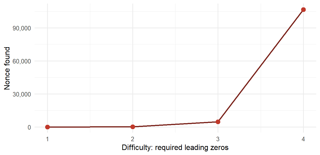
Hashes are fast to compute, so hashing alone does not make history expensive to rewrite. Proof-of-work adds a cost. A miner searches for a nonce such that the block hash satisfies a difficulty condition. In the teaching rule below, the hash must start with \(d\) zeros:
Verification is cheap because any node can hash the block once and check the leading zeros. Finding a valid nonce requires repeated trials.
This asymmetry is the key idea. Producing the proof is costly; checking it is cheap. In a financial ledger, that asymmetry can be used to make accepted history costly to replace. The block remains visible and verifiable; the barrier is the amount of work needed to find an alternative valid chain.
ggplot(difficulty_table, aes(x = difficulty, y = nonce)) +geom_line(color ="#7B241C", linewidth =1) +geom_point(color ="#C0392B", size =3) +scale_x_continuous(breaks = difficulty_table$difficulty) +scale_y_continuous(labels = scales::comma) +labs(x ="Difficulty: required leading zeros", y ="Nonce found")
Figure 7.5: Proof-of-work trials under increasing teaching difficulty.
The exact nonce depends on the block content, but the figure shows why difficulty matters: adding required leading zeros turns hashing into repeated search. Verification still requires a single hash check.
Bitcoin is the canonical proof-of-work case. Miners gather valid transactions, construct candidate blocks, search for a valid nonce, and broadcast the block when the proof is found. Ethereum is useful as a contrast because it moved from proof-of-work to proof-of-stake in 2022. This chapter keeps proof-of-work because it makes the cost of rewriting history visible in a small R example.
Transactions and fees
Transactions are the financial content of blocks. A pending transaction has a sender, receiver, amount, and fee. The fee compensates the block producer for including the transaction.
In this teaching model, rejection has three sources: insufficient sender balance, invalid amount or fee, and limited block capacity. The first is an accounting failure, the second is a rule failure, and the third is a scarcity problem.
# A tibble: 5 × 5
  tx_id sender receiver amount   fee
  <chr> <chr>  <chr>     <dbl> <dbl>
1 tx1   Alice  Bob          25  0.4
2 tx2   Bob    Carol        20  0.15
3 tx3   Carol  Alice        12  0.8
4 tx4   Dave   Bob          12  0.3
5 tx5   Alice  Carol        70  0.6
In many blockchain systems, transactions waiting for inclusion sit in a pending pool. A block producer may prefer transactions with higher fees, subject to validity and block capacity. If the block can include \(m\) transactions, a simple selection rule is:
# A tibble: 5 × 6
  tx_id sender receiver amount   fee status
  <chr> <chr>  <chr>     <dbl> <dbl> <chr>
1 tx3   Carol  Alice        12  0.8  Accepted
2 tx5   Alice  Carol        70  0.6  Accepted
3 tx1   Alice  Bob          25  0.4  Accepted
4 tx4   Dave   Bob          12  0.3  Rejected
5 tx2   Bob    Carol        20  0.15 Rejected
Code
block_selection$balances
# A tibble: 5 × 2
  wallet balance
  <chr>    <dbl>
1 Alice     16
2 Bob       60
3 Carol     72.2
4 Dave       5
5 Miner      1.8
The first output records the inclusion decision; the second output records the resulting balances. The accepted transactions are valid under the balance rule and fit inside the block capacity. The rejected transactions fail validation or remain outside the limited block space. The economic intuition is already visible: users pay for inclusion, and block producers respond to those incentives.
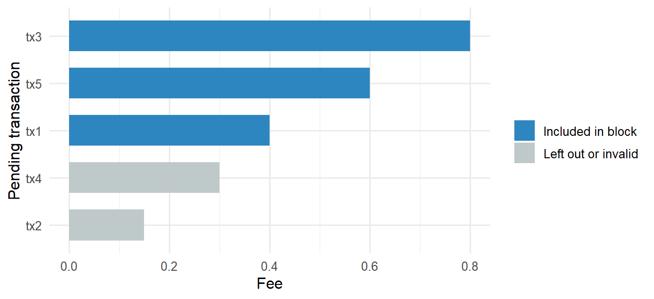
Code
fee_competition <- pending_transactions |>mutate(status =if_else(tx_id %in% block_selection$accepted$tx_id,"Included in block", "Left out or invalid"),tx_id =reorder(tx_id, fee) )ggplot(fee_competition, aes(x = tx_id, y = fee, fill = status)) +geom_col(width =0.65) +coord_flip() +scale_fill_manual(values =c("Included in block"="#2E86C1","Left out or invalid"="#BFC9CA")) +labs(x ="Pending transaction", y ="Fee", fill ="")
Figure 7.6: Fee ranking and block inclusion in a small pending pool.
This turns block construction into a market for scarce inclusion. The fee is small relative to the transfer amount, but it can decide timing when many transactions compete for limited capacity. Pending transactions, fees, and inclusion delays therefore reveal pressure on the settlement layer.
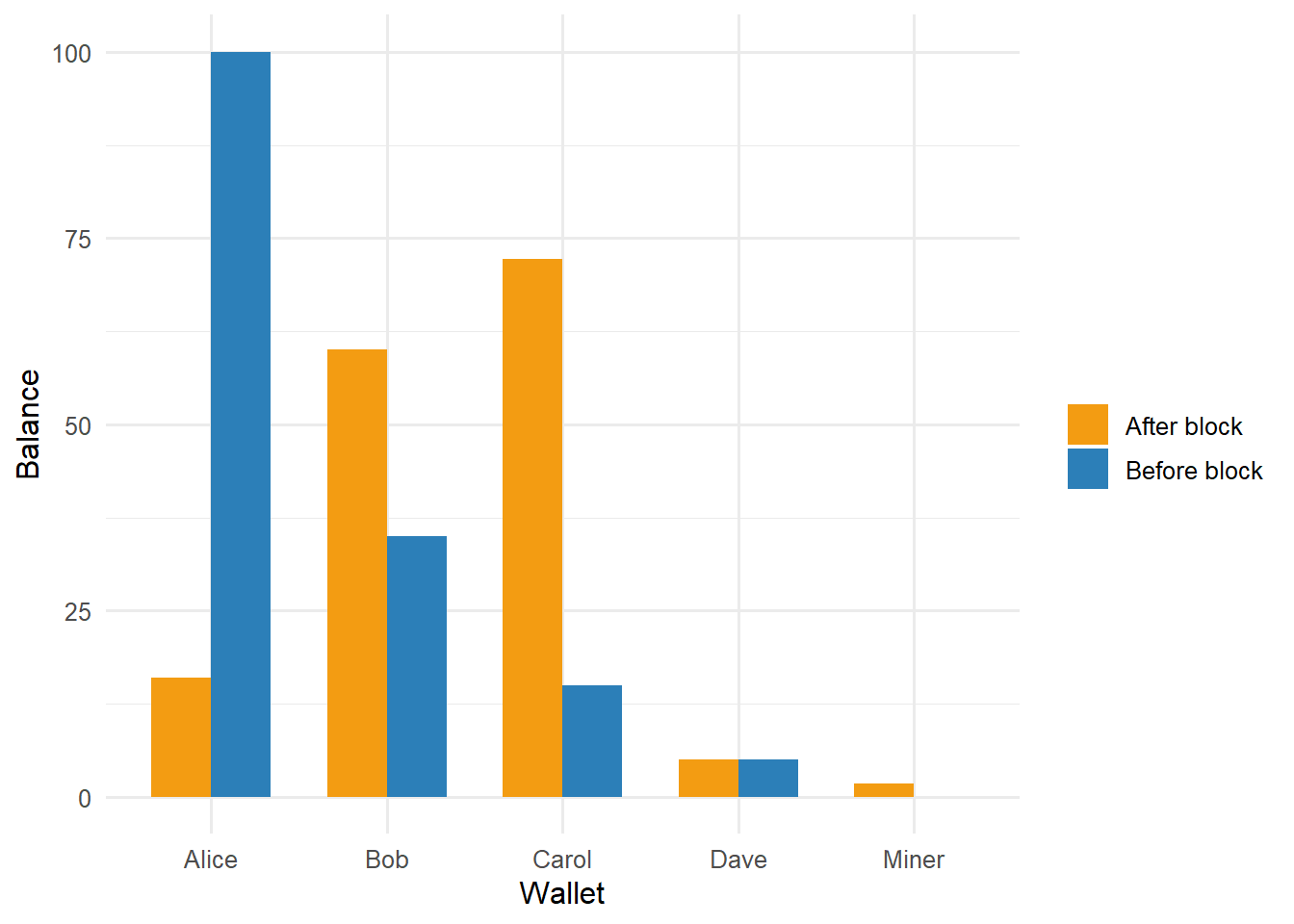
Code
balance_plot <-bind_rows(mutate(balances, state ="Before block"),mutate(block_selection$balances, state ="After block"))ggplot(balance_plot, aes(x = wallet, y = balance, fill = state)) +geom_col(position ="dodge", width =0.68) +scale_fill_manual(values =c("Before block"="#2C7FB8","After block"="#F39C12")) +labs(x ="Wallet", y ="Balance", fill ="")
Figure 7.7: Wallet balances before and after the mined block.
The balance plot connects block inclusion to state change. Senders lose the amount plus fee, receivers gain the transferred amount, and the next formula isolates the miner’s fee reward in this simplified example:
In Bitcoin, miners can also receive a block subsidy according to the issuance schedule. In this teaching account-based model, only transaction fees are shown.
Mining a transaction block
The accepted transactions can now become block data. The block hash commits to the transaction set, the parent hash, the timestamp, and the nonce.
The summary keeps the mined block readable while preserving the pieces that matter for validation: transaction count, nonce, parent hash, block hash, and chain status.
Changing a transaction after the block is mined breaks the chain.
This example connects pending transactions, balances, and the accepted ledger state. The hash commits to the candidate block; validation rules, signatures, balance checks, consensus, and network acceptance determine which transactions enter the ledger.
It also separates two views of the same system. The transaction view asks which transfers are accepted. The state view asks what the balances are after those transfers. Financial applications need both: history for auditability and state for valuation, reporting, and risk controls.
Digital signatures
A transaction also needs authorization. The ledger can define valid balances, fees, and block rules, but it still needs evidence that the owner of the value approved the transfer. Public-key cryptography supplies that authorization layer.
The basic object is a key pair:
\[
(\mathrm{sk}, \mathrm{pk}),
\]
where \(\mathrm{sk}\) is the private key and \(\mathrm{pk}\) is the public key. The private key must be kept secret. The public key can be shared because it is used for verification. A simplified signature workflow is:
\[
m = \mathrm{serialize}(\mathrm{transaction}),
\qquad
h = H(m),
\qquad
\sigma = \mathrm{Sign}_{\mathrm{sk}}(h),
\]
This gives two properties that matter for a financial ledger:
authenticity: the signature matches the public key associated with the spending authority;
integrity: changing the signed message invalidates the signature.
The ledger question is narrow and powerful: did the holder of the relevant private key authorize this exact transaction message? That question is smaller than legal identity, investor eligibility, tax treatment, or the existence of an off-chain asset. Those issues require identity, legal, operational, and governance layers around the cryptographic system.
The code below should be read as one security workflow:
create a key pair;
sign an exact transaction message;
verify the signature with the public key;
alter the message and see verification fail;
separate signature logic from confidentiality.
The next example uses RSA keys through the openssl package. This is a teaching choice. Bitcoin signatures use elliptic-curve schemes, including ECDSA over secp256k1 and Schnorr signatures for Taproot outputs. The teaching idea is the same: one key signs, the corresponding public key verifies, and any change to the signed message breaks verification.
The private key is the sensitive asset. The public key can travel through the network because it is used to check signatures. A wallet, custodian, or exchange may manage this key material for a user, but the economic implication is the same: control of the private key controls the ability to authorize spending.
# A tibble: 1 × 2
  message                     valid_signature
  <chr>                       <lgl>
1 Original signed transaction TRUE
Now alter the transaction and verify the old signature against the altered message. The amount and fee are unchanged, but the receiver changes from Bob to Carol.
The altered message fails verification. This is why signatures are part of the financial logic of a blockchain: the ledger should only accept transactions authorized by the holder of the relevant private key.
Confidentiality and encryption
Signatures and encryption solve different problems. A signature answers who authorized a message and whether the message changed. Encryption hides message contents from parties that do not hold the decryption key.
In a public-key encryption system, a sender can encrypt a message with the receiver’s public key. The receiver decrypts it with the receiver’s private key:
\[
c = \mathrm{Enc}_{\mathrm{pk}_B}(m),
\qquad
m = \mathrm{Dec}_{\mathrm{sk}_B}(c).
\]
Bitcoin transactions are usually public enough for network validation, so ordinary transaction data is visible to nodes. The encryption example below is therefore a teaching example for confidentiality. It clarifies why a private key is valuable: the key can authorize messages through signatures and can decrypt messages that were encrypted to the matching public key.
Code
bob_key <-rsa_keygen(bits =2048)bob_public_key <- bob_key$pubkeypayment_note <-charToRaw("Alice pays Bob 10 with fee 0.1")cipher_text <-rsa_encrypt(payment_note, bob_public_key)recovered_note <-rsa_decrypt(cipher_text, bob_key)tibble(object =c("Plain message", "Encrypted message", "Recovered message"),bytes =c(length(payment_note), length(cipher_text), length(recovered_note)),readable =c(rawToChar(payment_note), "<cipher text>", rawToChar(recovered_note)))
# A tibble: 3 × 3
  object            bytes readable
  <chr>             <int> <chr>
1 Plain message        30 Alice pays Bob 10 with fee 0.1
2 Encrypted message   256 <cipher text>
3 Recovered message    30 Alice pays Bob 10 with fee 0.1
The encrypted message is longer and unreadable as ordinary text. The receiver’s private key recovers the original message.
# A tibble: 1 × 2
  check                              valid
  <chr>                              <lgl>
1 Recovered message matches original TRUE
In production systems, large messages are commonly encrypted with a symmetric key, and the symmetric key is protected with public-key encryption. The small RSA example is still useful because it separates three ideas that are often mixed together:
Object
Main question
Financial meaning
Hash
Did the data change?
Integrity and compact commitment
Signature
Who authorized this exact data?
Spending authority and non-repudiation in the ledger model
Encryption
Who can read the data?
Confidentiality and access control
Private-key custody
Who can use the secret key?
Operational control over value
This separation matters for blockchain finance. A public ledger can allow verification while still creating privacy problems. A signature can prove that a key authorized a transaction while leaving the real-world owner of the key uncertain. Encryption can protect message contents while leaving metadata, timing, amounts, or network relationships exposed.
Custody and key risk
Private-key custody turns cryptography into a financial risk. If the private key is stolen, an attacker can authorize transfers. If the private key is lost, the owner may lose the ability to spend. If a custodian controls the private key, the user faces operational, legal, and counterparty risk. These risks are different from market risk, but they can dominate the financial outcome.
Code
custody_scenarios <-tibble(scenario =c("Self-custody","Lost private key","Stolen private key","Exchange custody","Two-of-three multisignature" ),who_can_sign =c("The holder of the wallet key","Nobody, if the key cannot be recovered","The attacker","The exchange or custodian","Any two authorized key holders" ),main_financial_risk =c("Operational mistakes by the owner","Permanent loss of spending ability","Unauthorized transfer","Counterparty, legal, and operational failure","Coordination failure or compromised signers" ))custody_scenarios
# A tibble: 5 × 3
  scenario                    who_can_sign                   main_financial_risk
  <chr>                       <chr>                          <chr>
1 Self-custody                The holder of the wallet key   Operational mistak…
2 Lost private key            Nobody, if the key cannot be … Permanent loss of …
3 Stolen private key          The attacker                   Unauthorized trans…
4 Exchange custody            The exchange or custodian      Counterparty, lega…
5 Two-of-three multisignature Any two authorized key holders Coordination failu…
Multisignature arrangements are one way to reduce single-key failure. A two-of-three setup can require any two authorized keys to sign before funds move. That design changes the operational problem from protecting one secret to coordinating several secrets. It can reduce theft and loss risk, but it adds governance and recovery procedures.
For this chapter, the important point is that security is part of the financial model. The ledger state says who controls value according to protocol rules. The signature says which key authorized a transaction. Custody determines who can use that key in practice. Privacy determines how much of the transfer history can be linked to people, institutions, or strategies.
Network and consensus
A blockchain ledger is distributed over a peer-to-peer network. A simplified proof-of-work workflow is:
users broadcast transactions;
nodes check transaction validity;
miners gather valid pending transactions into candidate blocks;
miners search for a proof-of-work;
the first valid block is broadcast;
nodes accept the block if the proof and the transactions are valid;
new blocks build on the accepted parent hash.
The same workflow can be represented as a graph. Let \(a_{ij}=1\) when a message can move from node \(i\) to node \(j\), and \(a_{ij}=0\) otherwise. A simple measure of local connectivity is the total degree:
\[
d_i = \sum_j a_{ij} + \sum_j a_{ji}.
\]
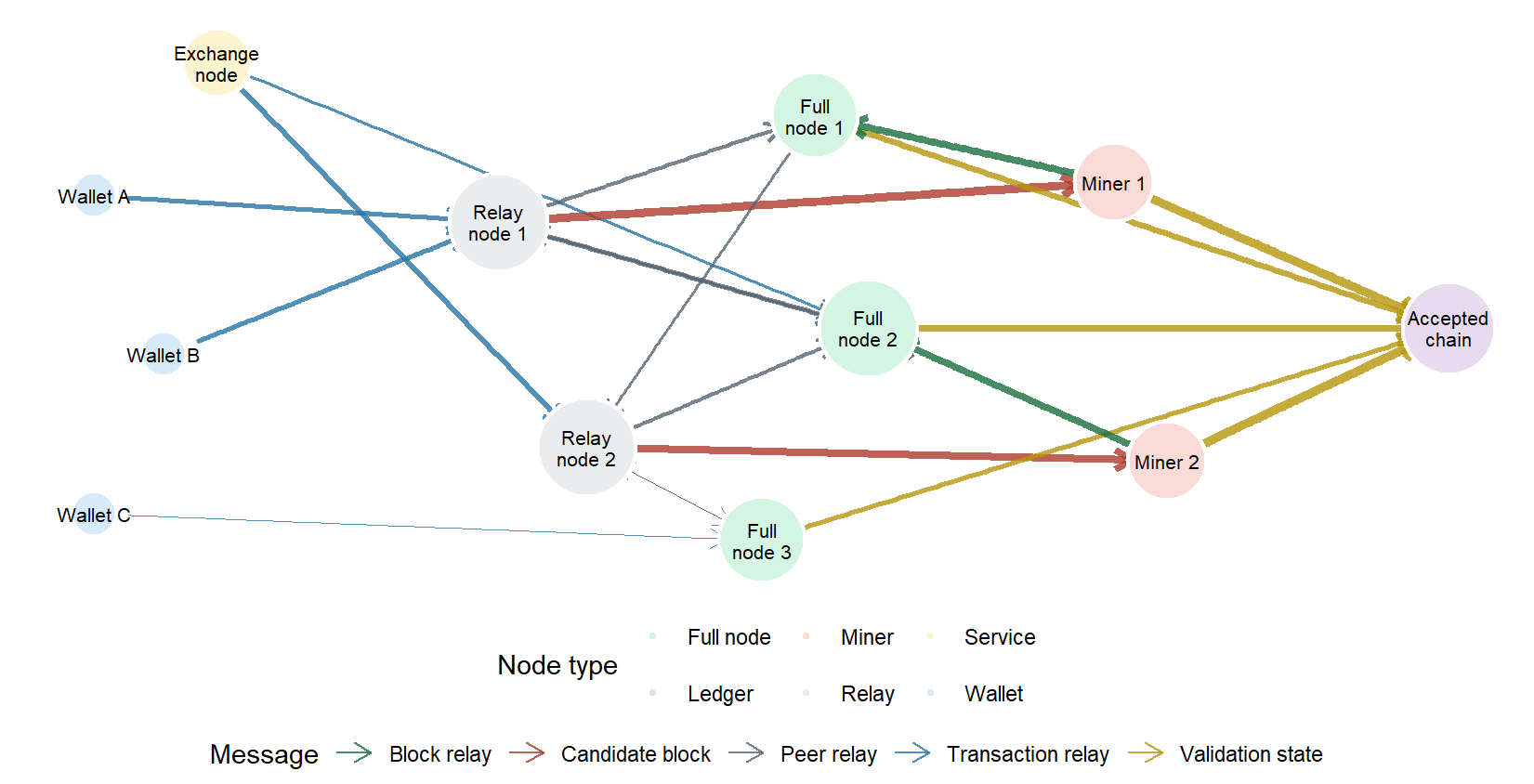
In the next figure, node size is proportional to \(d_i\). Wallets are peripheral, while relay, full-node, and mining nodes sit closer to the center of message propagation.
Figure 7.8: A simplified peer-to-peer blockchain network.
The diagram shows how ledger validity depends on message propagation. Wallets and service nodes inject transactions from the edge of the graph. Relay and full nodes move messages across the network. Miners receive candidate transactions, propose blocks, and broadcast block information back to validating nodes. The accepted chain is the history that nodes are willing to extend after verification.
The useful part of this graph is the topology. The same transaction can reach the accepted ledger through several paths, and nodes with more connections have more influence over propagation. A valid transaction still has to move through a communication layer before it becomes part of the history that participants observe.
Consensus is the rule that tells nodes which valid history to extend. In Bitcoin, the accepted history is tied to accumulated proof-of-work. The economic security argument is that rewriting history requires controlling enough computational work to replace the accepted chain, which is costly.
Incentives complete the mechanism. Fees and block rewards encourage miners to spend resources on valid blocks. Invalid blocks waste effort because nodes reject them.
The generic lab now has enough pieces to read Bitcoin more carefully:
Toy mechanism
Bitcoin object
Financial reading
Account balance table
UTXO set reconstructed from unspent outputs
Spendable value controlled by keys
Toy transaction
Signed transaction with inputs, outputs, and fee
Payment instruction and settlement cost
Block with parent hash
Block header linked to the previous block
Commitment to accepted history
Toy proof-of-work difficulty
Network difficulty target
Cost of rewriting recent settlement
Fee reward
Fees plus protocol-defined subsidy
Miner incentive and block-space allocation
Peer-to-peer message graph
Wallets, relays, full nodes, miners, and services
Propagation, validation, and observability
7.3 Bitcoin case: a proof-of-work ledger
With that map in place, Bitcoin can be read as a specific monetary and payment system built from ledger, hash, signature, network, and proof-of-work pieces. Its design connects payments, scarce issuance, public verification, private-key custody, and costly history rewriting (Nakamoto 2008).
The generic model and Bitcoin share the same broad workflow:
The bridge above gives the correspondence. The main simplifications are:
Generic model in this chapter
Bitcoin case
Account balances are stored directly for teaching clarity
Balances are inferred from unspent transaction outputs
Transactions move amounts from sender to receiver
Transactions consume previous outputs and create new outputs
The miner receives transaction fees in the teaching balance table
Miners can receive fees and a protocol-defined block subsidy
Difficulty is a small number of leading zeros
Difficulty adjusts so blocks arrive near the protocol target interval
Finality is shown as a valid chain in R
Settlement confidence grows as more blocks build on top
A table also helps separate protocol roles from market access roles:
Role
Protocol or market function
Financial reading
Wallet
Creates and signs transactions
Custody and spending authority
Mempool
Holds valid pending transactions before block inclusion
Fee pressure and settlement delay
Miner
Selects transactions and searches for proof-of-work
Incentives and block-space allocation
Full node
Verifies blocks and transactions against consensus rules
Independent validation
Accepted chain
Stores the history participants extend
Settlement reference
Exchange or custodian
Provides market access and often manages keys
Counterparty and operational risk
Explorer or analytics tool
Makes public transaction data searchable
Monitoring, attribution, and compliance
This table separates protocol roles from financial access roles. A price, a wallet balance, a transaction status, and an exchange account are produced by different parts of the system. Treating them as one object makes Bitcoin look flatter than it is.
A Bitcoin transaction also has an operational path:
Stage
Mechanism
Financial consequence
Wallet construction
The wallet selects spendable outputs, creates new outputs, and signs the transaction
Spending authority and fee choice
Mempool relay
Nodes hold valid pending transactions according to local policy
Pending settlement and public fee pressure
Block construction
Miners select transactions subject to block weight and fee incentives
Scarce block space
Coinbase transaction
The miner includes a special transaction that pays the subsidy and collected fees
Miner revenue and issuance rule
Confirmation
The transaction is included in a block, then new blocks build above it
Increasing settlement confidence
Fee-rate thinking is useful because block space is measured by transaction size as well as by amount paid. A compact model is:
Miners compare valid pending transactions under block-space constraints, so a large transaction may need a larger absolute fee to offer the same fee rate as a smaller transaction. The miner’s block revenue combines the protocol-defined subsidy and the fees from included transactions:
The subsidy follows the issuance schedule, while the fee component changes with demand for block space. This is why mempool conditions, fee rates, and confirmation depth are financial variables, even before looking at the market price of bitcoin.
The account-based model says that Alice has a balance and can send part of it. Bitcoin uses a UTXO model. A UTXO is an unspent transaction output. If Alice controls previous outputs worth 0.8 BTC and 0.4 BTC, and wants to pay 0.9 BTC, her transaction spends enough previous outputs and creates new outputs: one for the receiver, one for change back to Alice, and one implicit fee to the miner. The balance is therefore reconstructed from the set of unspent outputs controlled by Alice’s keys.
In the account example above, the fee was an explicit column. Here the fee is the unassigned remainder after inputs and outputs are compared. The economic meaning is similar: the sender gives up value, the receiver obtains value, and the miner has an incentive to include the transaction.
The same example can be read as a small UTXO table:
Side
Reference
Amount (BTC)
Controlled by
Role
Input
Previous output 1
0.80
Alice key
Spent source of value
Input
Previous output 2
0.40
Alice key
Spent source of value
Output
New output 1
0.90
Bob key
Payment to receiver
Output
New output 2
0.28
Alice key
Change back to sender
Fee
Implicit remainder
0.02
Miner
Incentive for inclusion
The table balances because inputs of 1.20 BTC fund outputs of 1.18 BTC and an implicit fee of 0.02 BTC. After the transaction is accepted, the two previous outputs are spent, and only the new outputs remain available for future transactions.
Bitcoin transactions as a network
A UTXO ledger can also be read as a network. Nodes represent wallets, addresses, services, or output clusters. Directed edges represent value moving from one node to another. The edge weight can be the BTC amount. This view is useful because it changes the question from a single payment to a system of relationships: which nodes concentrate flow, which nodes mostly receive, which nodes mostly distribute, and where fees or change outputs appear.
The next example uses a small synthetic transaction network. It is not meant to identify real addresses. Its purpose is to show how network tools can turn ledger data into a visual model. This is the point where the chapter moves from blockchain as a validation mechanism to blockchain as analyzable financial data.
Figure 7.9: A synthetic UTXO transaction network with BTC-weighted flows.
The network view carries a different kind of explanation. The exchange and the miner appear as high-flow nodes because several edges pass through them. Alice creates both a payment edge and a change edge. The fee pool collects small edges that would be easy to miss in a table. A merchant receives payments and later settles part of the balance back to an exchange. These are financial roles, even in a synthetic network.
This figure should be read as an accounting map. The edge width shows value, the edge color shows transaction role, and the node size shows total flow handled by each participant. It makes three concepts visible at once: issuance through the coinbase reward, payments through wallet-to-merchant edges, and operational concentration through the exchange and miner nodes.
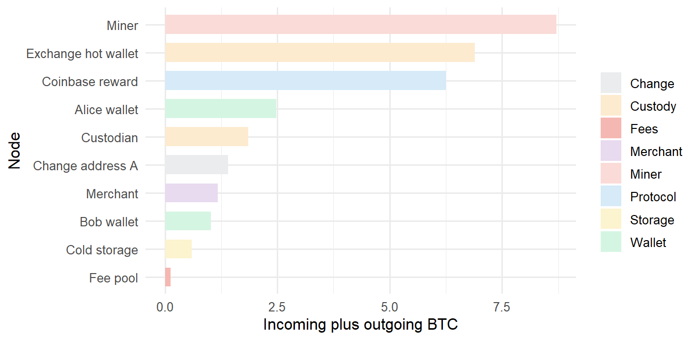
We can summarize the same graph numerically. Let \(w_{ij}\) be the BTC value sent from node \(i\) to node \(j\). The incoming and outgoing value of node \(i\) are:
network_node_summary |>mutate(node =reorder(node, total_value)) |>ggplot(aes(x = node, y = total_value, fill = type)) +geom_col(width =0.68) +coord_flip() +scale_fill_manual(values =c("Protocol"="#D6EAF8","Miner"="#FADBD8","Custody"="#FDEBD0","Wallet"="#D5F5E3","Merchant"="#E8DAEF","Change"="#EAECEE","Storage"="#FCF3CF","Fees"="#F5B7B1" )) +labs(x ="Node", y ="Incoming plus outgoing BTC", fill ="")
Figure 7.10: Incoming plus outgoing BTC by node in the synthetic UTXO network.
This is where network analysis becomes useful for financial interpretation. Large nodes can indicate custody, market access, mining income, payments, or operational concentration. The meaning depends on the node label and the transaction role. A high-flow exchange address has a different interpretation from a high-flow merchant or miner address.
The bar chart forces the visual claim into a simple metric. In the synthetic data, the miner and the exchange dominate total observed flow, while the fee pool is small in value but important for incentives. A real blockchain dataset would require address clustering, time windows, filtering rules, and careful labeling, but the modeling question is the same: which parts of the transaction graph carry the most economic activity?
Bitcoin also makes proof-of-work part of monetary security. A miner proposes a block and searches for a valid proof. Nodes verify the block by checking the proof, transaction validity, and the rule that spent outputs have not already been spent. A transaction with one confirmation is included in one block. More confirmations mean that additional blocks have been built on top of that block, raising the cost of replacing that history.
The settlement idea is probabilistic. A payment becomes harder to reverse as more proof-of-work accumulates above it. This is why confirmations matter in Bitcoin payments: they are a practical measure of how deeply a transaction sits inside the accepted history.
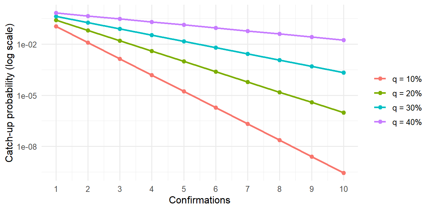
One simplified way to visualize the intuition is a catch-up race. Suppose an attacker controls share \(q\) of mining power, with \(0<q<0.5\), and an honest chain is already \(z\) confirmations ahead. A compact approximation for the probability that the attacker catches up is:
The approximation is a teaching device. It captures the central shape: when the attacker has less than half of total work, each additional confirmation lowers the catch-up probability.
Figure 7.11: Approximate catch-up probability by confirmations and attacker share.
The logarithmic scale makes the settlement intuition visible. Confirmations translate settlement depth into a practical risk measure: they express the cost of replacing recent history. The same payment can be operationally acceptable at different confirmation depths depending on amount, counterparty risk, liquidity needs, and the recipient’s tolerance for reversal risk.
Bitcoin is financially interesting for four reasons.
First, it turns ledger maintenance into an incentive problem. Miners spend resources because accepted blocks can pay rewards and fees. Second, it makes custody explicit: control of private keys is control over spending authority. Third, it creates a public audit trail, so anyone can verify the transaction history according to protocol rules. Fourth, it introduces a digital asset with a rule-based issuance schedule, which makes scarcity part of the protocol design.
The R model above should be read as a simplified map. It captures blocks, hashes, proof-of-work, fees, validation, and ledger updates. It leaves out many Bitcoin details: UTXO selection algorithms, script rules, block propagation, difficulty adjustment mechanics, mempool policy, fee estimation, wallet software, and network topology. The simplification is deliberate. The goal is to make the financial logic visible before adding production-level complexity.
7.4 Tokenization
Tokenization extends the ledger idea from native coins to other financial or economic claims. A token can represent a unit in a digital asset, a claim on a cash-flow arrangement, a fund share, a loyalty point, a stablecoin balance, or a record linked to an off-chain asset. The crucial point is that the token record and the legal or operational claim have to be aligned.
The shift from Bitcoin to tokenization changes the financial question. In Bitcoin, the native asset and the ledger are part of the same protocol. In tokenization, the ledger records ownership units whose value often depends on something outside the ledger: cash, securities, real assets, fund shares, invoices, commodities, or contractual rights. That creates two layers:
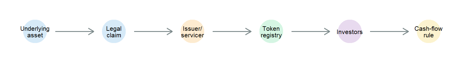
Layer
Question
On-chain record
Who holds how many tokens according to the ledger?
Off-chain claim
What legal, economic, or operational right does each token represent?
The on-chain record can be precise while the off-chain claim still requires legal documentation, custody, audits, servicing, redemption rules, and dispute resolution. This is why tokenization is a finance topic as much as a technology topic.
Figure 7.12: Tokenization layers from off-chain asset to cash-flow rule.
This stack is where tokenization becomes a financial structure. The token registry can say who holds units. Valuation and risk also depend on the asset, legal claim, servicing process, transfer restrictions, and cash-flow rule. A token model is incomplete unless the financial claim represented by the token is explicit.
In a simple model, a token contract has:
an issuer;
a token name;
total supply;
holder balances;
transfer rules;
optional cash-flow or redemption rules.
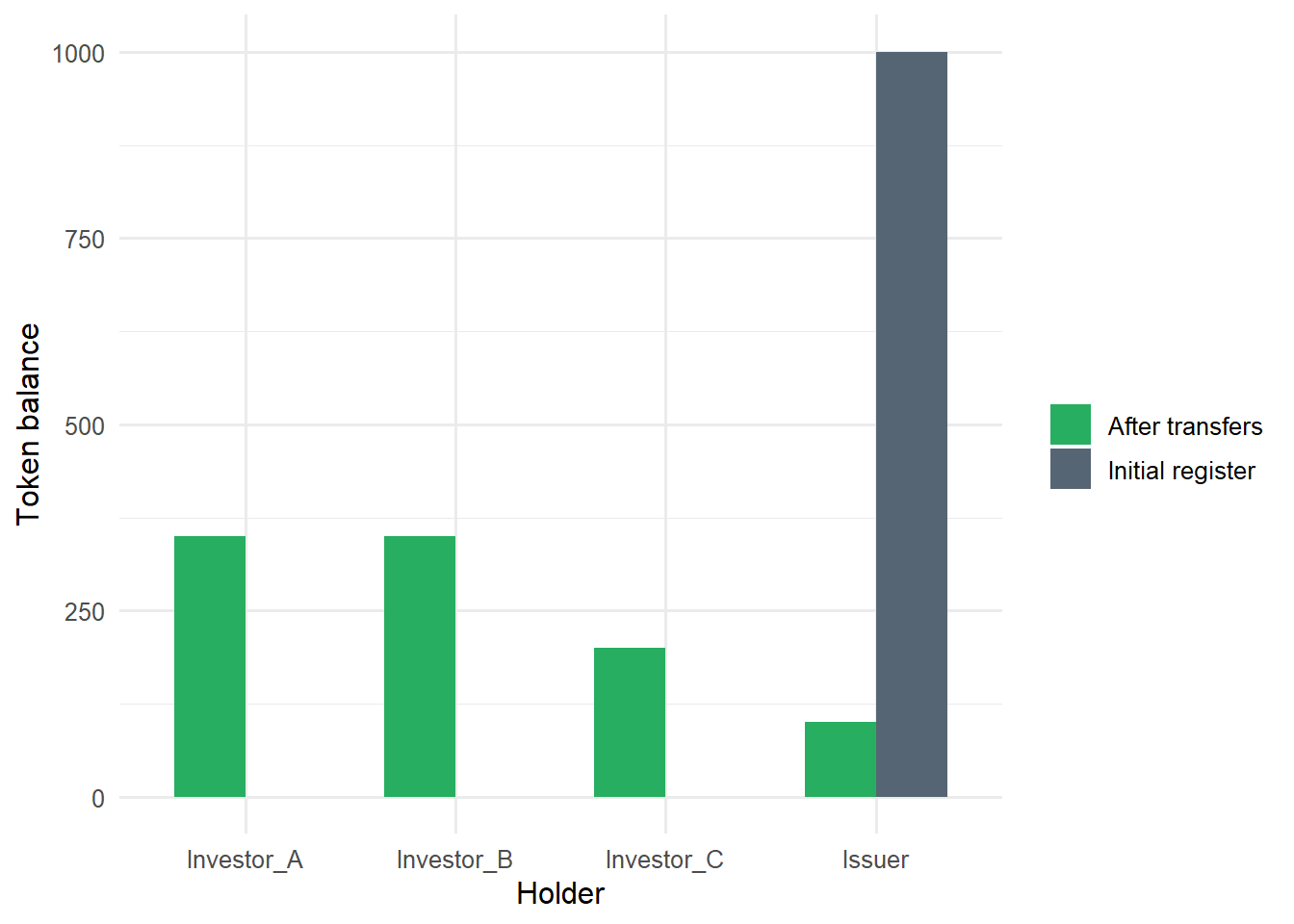
Suppose a hypothetical issuer creates 1,000 tokens linked to participation in a small financial asset pool.
Code
token_metadata <-tibble(token ="POOL_A_TOKEN",underlying ="Hypothetical asset-pool participation",total_supply =1000,unit_claim ="1 token = 0.1% of the pool cash-flow rule")token_register <-tibble(holder =c("Issuer", "Investor_A", "Investor_B", "Investor_C"),token_balance =c(1000, 0, 0, 0))token_metadata
token_plot <-bind_rows(mutate(token_register, state ="Initial register"),mutate(token_register_after, state ="After transfers"))ggplot(token_plot, aes(x = holder, y = token_balance, fill = state)) +geom_col(position ="dodge", width =0.68) +scale_fill_manual(values =c("Initial register"="#566573","After transfers"="#27AE60")) +labs(x ="Holder", y ="Token balance", fill ="")
Figure 7.13: Token ownership before and after transfers.
The plot separates issuance from redistribution. The issuer begins with the full supply, and later balances show which investors would receive cash flows under a proportional allocation rule.
If the pool distributes cash flow \(C\), a proportional token rule allocates:
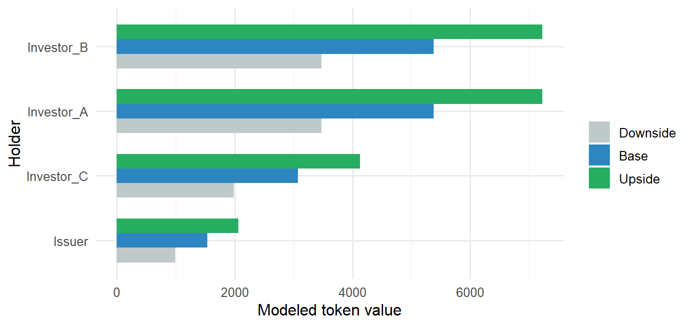
The same register can be connected to valuation. If the token represents a proportional claim on expected cash flows \(C_t\), and \(r\) is the discount rate, then holder \(h\) has a model value:
This is a simple discounted cash-flow model. The blockchain register tells us the token balance. The valuation model still needs expected cash flows, discount rates, legal enforceability, and servicing assumptions.
holder_token_value |>mutate(holder =reorder(holder, holder_value)) |>ggplot(aes(x = holder, y = holder_value, fill = scenario)) +geom_col(position ="dodge", width =0.68) +coord_flip() +scale_fill_manual(values =c("Downside"="#BFC9CA","Base"="#2E86C1","Upside"="#27AE60" )) +labs(x ="Holder", y ="Modeled token value", fill ="")
Figure 7.14: Scenario value of the tokenized cash-flow claim.
The valuation figure is deliberately simple. It shows that a token register and a valuation model answer different questions. The register answers who holds units. The cash-flow model asks what those units may be worth under a set of assumptions. Tokenization becomes financially meaningful when those two layers are kept aligned.
This example shows why tokenization belongs in a financial modeling course. It combines a ledger, ownership units, transfer rules, cash-flow allocation, and valuation. The hard parts appear quickly: custody, investor rights, transfer restrictions, identity checks, tax treatment, legal enforceability, valuation, and operational controls.
7.5 Privacy
Public blockchains make verification easier by exposing transaction history, but that transparency creates privacy questions. A public address can be pseudonymous, yet transaction patterns may still reveal relationships. If an address is linked to a person or institution, past and future activity can become easier to trace.
The banking model usually limits transaction information to the parties, the bank, and regulators. A public blockchain makes more information visible to the network. Privacy-preserving tools, address management, zero-knowledge proofs, and permissioned ledgers are attempts to balance auditability and privacy.
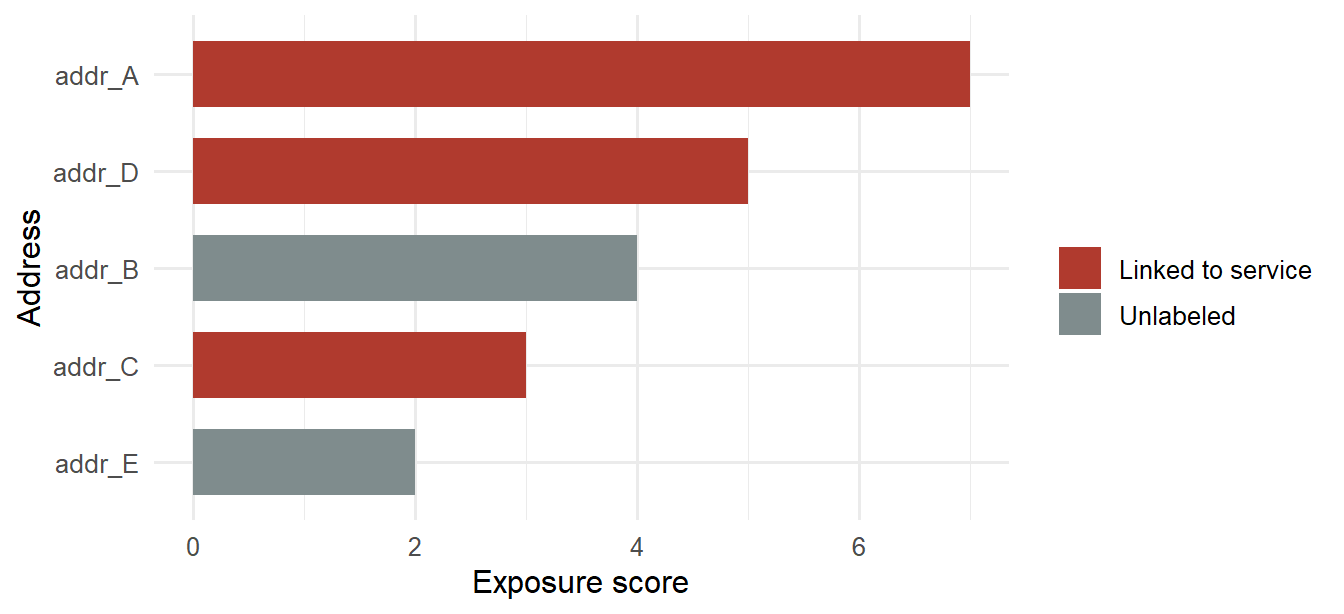
For modeling purposes, privacy can be treated as a linkage problem. A public address may start without a real-world name, but repeated use, counterparties, service labels, timing, and transaction amounts can make the address easier to classify. A simple exposure score for address \(a\) can be written as:
where \(\mathrm{ServiceLabel}_a\) equals one when the address has been linked to a known service such as an exchange, custodian, merchant, or public donation address.
privacy_summary |>mutate(address =reorder(address, exposure_score),service_status =if_else(labeled_service ==1,"Linked to service", "Unlabeled") ) |>ggplot(aes(x = address, y = exposure_score, fill = service_status)) +geom_col(width =0.68) +coord_flip() +scale_fill_manual(values =c("Linked to service"="#B03A2E","Unlabeled"="#7F8C8D")) +labs(x ="Address", y ="Exposure score", fill ="")
Figure 7.15: Address exposure score in a small public-ledger example.
The chart makes the linkage problem easier to see. Addresses with repeated activity, many counterparties, and service labels rise in the exposure ranking. This kind of score can guide monitoring, clustering, and privacy-risk review. It should not be read as proof of identity by itself.
The score is a teaching device, but the logic is important. Address reuse and public service labels reduce ambiguity. A blockchain can be transparent enough for audit and still expose sensitive relationships, strategies, or customer activity. This is why privacy is a financial design issue: disclosure affects trading behavior, institutional adoption, compliance, and personal safety.
Privacy tools change the tradeoff. Address rotation can reduce simple reuse. Coin-control policies can reduce accidental linkage. Zero-knowledge proofs can allow verification of selected statements while hiding underlying transaction details. Permissioned ledgers can restrict who sees transaction data. Each choice changes auditability, compliance cost, market confidence, and the amount of information available for analysis.
7.6 Advantages and limits
The chapter’s main lesson is that blockchain is a design for financial records and transfers. Its interest comes from combining records, verification, incentives, custody, privacy, and settlement rules in one system. Bitcoin shows the native-asset case: the ledger, asset, issuance rule, and settlement process belong to the same protocol. Tokenization shows a different use: the ledger records units whose value may depend on legal claims, servicing, and assets outside the ledger.
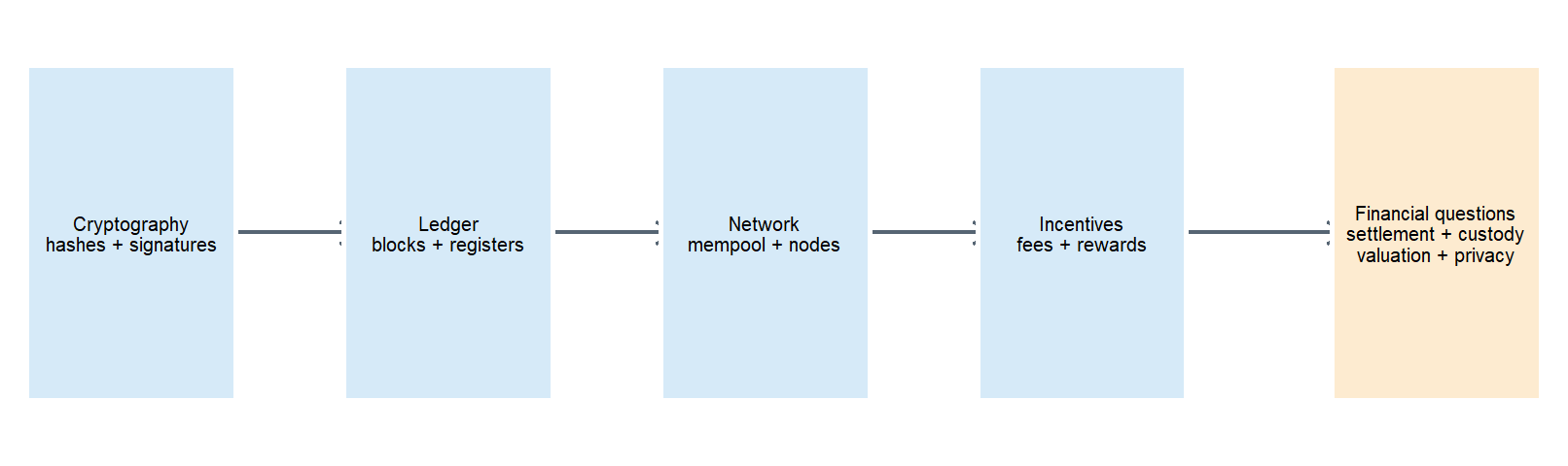
Figure 7.16: Blockchain mechanisms and financial modeling questions.
The figure summarizes the modeling move in the chapter. Technical mechanisms matter because they change financial questions: who can authorize a transfer, which history is accepted, how quickly transactions settle, what incentives shape block inclusion, how token claims are valued, and how much information is visible to others.
Potential advantages include:
shared audit trail;
public verification of ledger history;
resistance to undetected alteration;
programmable transfers and token rules;
faster experimentation with digital assets and settlement logic.
Important limits include:
scalability and transaction cost;
privacy leakage;
governance disputes;
custody risk from lost or stolen private keys;
smart-contract or implementation errors;
regulatory uncertainty;
weak links between on-chain tokens and off-chain assets.
The strongest way to read blockchain in this book is as a special application of financial modeling. Prices, returns, portfolios, and VaR model market behavior. Blockchain models the record-keeping and transfer layer of financial value. A private key changes who can authorize a payment. A fee changes which transactions may be included sooner. A confirmation changes settlement risk. A token rule changes who receives cash flows. A privacy design changes who can observe financial relationships. Small technical choices can therefore change the financial meaning of the system.
This makes the chapter a bridge from market models to financial infrastructure. It asks how value is authorized, recorded, transferred, observed, and sometimes tokenized. That question is narrower than the full universe of digital assets, but it is rich enough to connect computation, cryptography, networks, and finance in one modeling problem.
7.7 Further visual resources
The following resources are optional visual complements. They are most useful after the R examples, when the reader already has the ledger, hash, signature, network, and privacy objects in mind.