The previous chapter estimated return exposures one asset at a time. Portfolio allocation turns those individual assets into a portfolio decision. The practical question is how much capital should be assigned to each asset when expected returns, risk, correlations, and investment constraints are considered together.
Optimization selects a feasible solution under an explicit objective and a set of constraints. In this chapter, the feasible solution is a vector of portfolio weights. The objective can be low risk, high expected return, a strong return-risk ratio, or a benchmark comparison. The constraints can require full investment, long-only positions, maximum weights, minimum weights, or rebalancing rules. R is useful because the calculation combines data transformation, matrix operations, optimization, and performance evaluation.
Diversification is the central idea. If all assets move together, portfolio risk remains close to single-asset risk. If assets respond differently to common shocks, portfolio volatility can fall even when expected return remains attractive. The correlation examples from earlier chapters prepare this point: co-movement determines how much risk can be reduced by combining assets.
The combined investment is a portfolio, and each percentage invested in an individual asset is a portfolio weight. Portfolio allocation models estimate or test these weights. The chapter separates four tasks: estimate returns and covariances, optimize weights under constraints, compare benchmarks, and evaluate realized performance. It starts with a single-period FANG portfolio, then compares optimization methods, examines an equally weighted benchmark, introduces synthetic assets to isolate diversification, and finishes with rebalancing and performance evaluation.
5.1 The single-period problem
The single-period problem is the simplest framework for portfolio allocation. At \(t=0\), the investor observes historical information, chooses portfolio weights, and then realizes a portfolio return at \(t=1\).
The example uses the PortfolioAnalytics package to distribute 100% of available capital across four stocks. For convenience, the example uses monthly returns from the FANG database.
If \(w_i\) is the portfolio weight of asset \(i\) and \(R_i\) is its return, the portfolio return is defined as
# A tibble: 192 × 3
# Groups:   symbol [4]
   symbol date       monthly.returns
   <chr>  <date>               <dbl>
 1 META   2013-01-31        0.106
 2 META   2013-02-28       -0.120
 3 META   2013-03-28       -0.0613
 4 META   2013-04-30        0.0856
 5 META   2013-05-31       -0.123
 6 META   2013-06-28        0.0218
 7 META   2013-07-31        0.479
 8 META   2013-08-30        0.122
 9 META   2013-09-30        0.217
10 META   2013-10-31       -0.000398
# ℹ 182 more rows
The PortfolioAnalytics package expects returns in a wide format, with one column per asset. The FANG_monthly_returns object is tidy, with a symbol column identifying the stock. The following transformation reshapes the data so each stock has its own return column.
The FANG information is the same, but the format now matches the requirements of the portfolio functions. The correlation matrix summarizes how the four stock returns move together.
The lowest correlation is between META and AMZN (0.1846197), which indicates a weak linear relationship. GOOG and AMZN have a correlation of 0.6171376, suggesting a stronger linear relationship between those stock returns. In principle, lower correlation creates greater diversification possibilities when forming a portfolio. The ice-cream and hot-chocolate example used a correlation of -0.9 to illustrate a strong volatility-reduction effect. In practice, strongly negative correlations are difficult to find, although diversification gains can arise whenever correlation is below +1.
The model output is a vector of weights, which indicates how much capital is assigned to each of the four assets.
The portfolio specification is defined with portfolio.spec().
Code
# Create the portfolio specificationport_spec <-portfolio.spec(colnames(fang))port_spec
**************************************************
PortfolioAnalytics Portfolio Specification
**************************************************

Call:
portfolio.spec(assets = colnames(fang))

Number of assets: 4
Asset Names
[1] "META" "AMZN" "NFLX" "GOOG"
The portfolio specification uses four assets. A full-investment constraint keeps the weights close to a total of 1. In practical terms, requiring an exact sum of 1 can be too restrictive for numerical optimization, so the allowed range is 0.99 to 1.01.
\[
0.99 \leq \sum_{i=1}^{N}w_i \leq 1.01.
\]
The add.constraint() function inserts this restriction into the portfolio specification.
Code
port_spec <-add.constraint(portfolio = port_spec, type ="weight_sum",min_sum =0.99, max_sum =1.01)port_spec
The chapter focuses on risk and return as a joint portfolio problem. The optimization setup adds objectives for expected return and standard deviation. The return per unit of risk used to compare portfolios is
\[
SR(w)=\frac{E(R_p)}{\sigma_p},
\quad \text{with } w \text{ subject to the constraints above.}
\]
Code
# Add an objective to minimize portfolio standard deviationport_spec <-add.objective(portfolio = port_spec,type ="risk",name ="StdDev")port_spec <-add.objective(portfolio = port_spec,type ="return",name ="mean")port_spec
The portfolio specification indicates that four assets are available: META, AMZN, NFLX, and GOOG. The constraints require the portfolio to invest 100% of the available funds, or very close to that value, and to keep individual weights nonnegative.
Removing the box constraint would allow the model to deliver negative portfolio weights. Negative portfolio weights represent short sales, which are positions that benefit when an asset price declines. Many investment mandates restrict short selling, so the box constraint makes the exercise closer to a long-only portfolio decision.
The optimize.portfolio() function can solve the portfolio problem with several methods, constraints, and objectives. The examples below compare the random and ROI methods.
The output above shows the portfolio weights, return, and risk of the two optimized portfolios. Before plotting the optimized results, the initial situation is inspected: the individual assets before considering any portfolio.
The relevant FANG data provide the individual monthly returns used to estimate the allocation.
# A tibble: 4 × 4
  symbol   mean     sd    sr
  <chr>   <dbl>  <dbl> <dbl>
1 AMZN   0.0257 0.0817 0.314
2 GOOG   0.0176 0.0594 0.296
3 META   0.0341 0.0989 0.345
4 NFLX   0.0592 0.167  0.355
Code
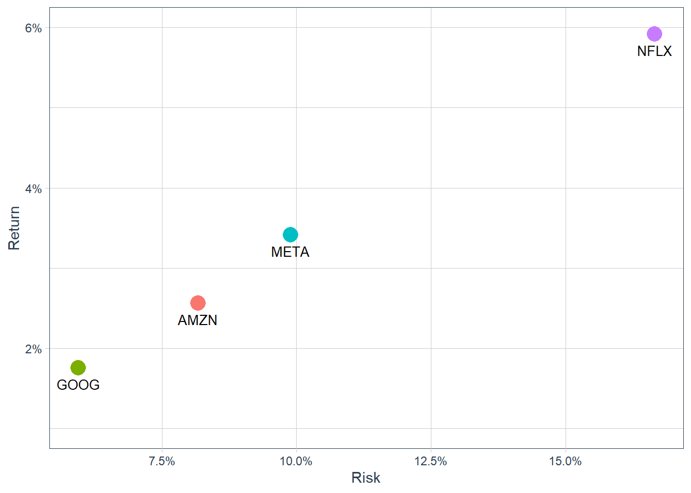
ggplot(FANG_stats, aes(x = sd, y = mean, color = symbol)) +geom_point(size =5) +geom_text(aes(label =paste0(symbol)),vjust =2, color ="black", size =3.5) +labs(x ="Risk", y ="Return") +scale_y_continuous(limits =c(0.01, 0.06),labels = scales::percent) +scale_x_continuous(labels = scales::percent) +theme_tq() +theme(legend.position ="none", legend.title =element_blank())
Figure 5.1: FANG, the four individual assets.
The plot places the four individual assets in mean-variance space. Portfolio allocation adds a portfolio perspective by combining assets so the joint risk-return profile can improve over a single-asset choice. The optimization process searches for the allocation that satisfies the objective and constraints.
For example, a portfolio with 3.5% monthly expected return and 15% standard deviation is dominated by alternatives with similar return and lower risk. A portfolio with 4% expected return and 5% risk would have a stronger return per unit of risk. This is the kind of comparison the optimizer formalizes.
Random portfolio optimization evaluates many candidate portfolios. Under the selected objective, the method searches for a combination with a more attractive return per unit of risk than the individual assets.
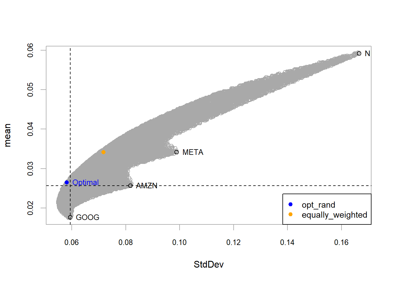
Figure 5.2: FANG, random method optimal portfolio.
According to the portfolio specification and asset universe, the gray circles represent feasible combinations of the individual assets. Some feasible portfolios have lower risk than GOOG. The algorithm selects the blue portfolio as the optimum under the chosen objective and constraints. This portfolio has approximately the same risk as GOOG with higher expected return, and a similar expected return to AMZN with lower risk. The gray portfolios form a mean-variance frontier. Portfolios to the left of that boundary are unavailable under the current data and constraints, and the selected optimum lies on the frontier.
The blue point marks the strongest available trade-off under the optimization setup. A point above it would offer higher return for the same risk, and a point to the left would offer lower risk for the same return. Those alternatives are outside the feasible set. Points below or to the right are feasible, although they offer a weaker trade-off. Efficient portfolios are therefore located on the upper-left boundary of the mean-variance cloud.
The corresponding weights translate the blue point into an implementable allocation.
Code
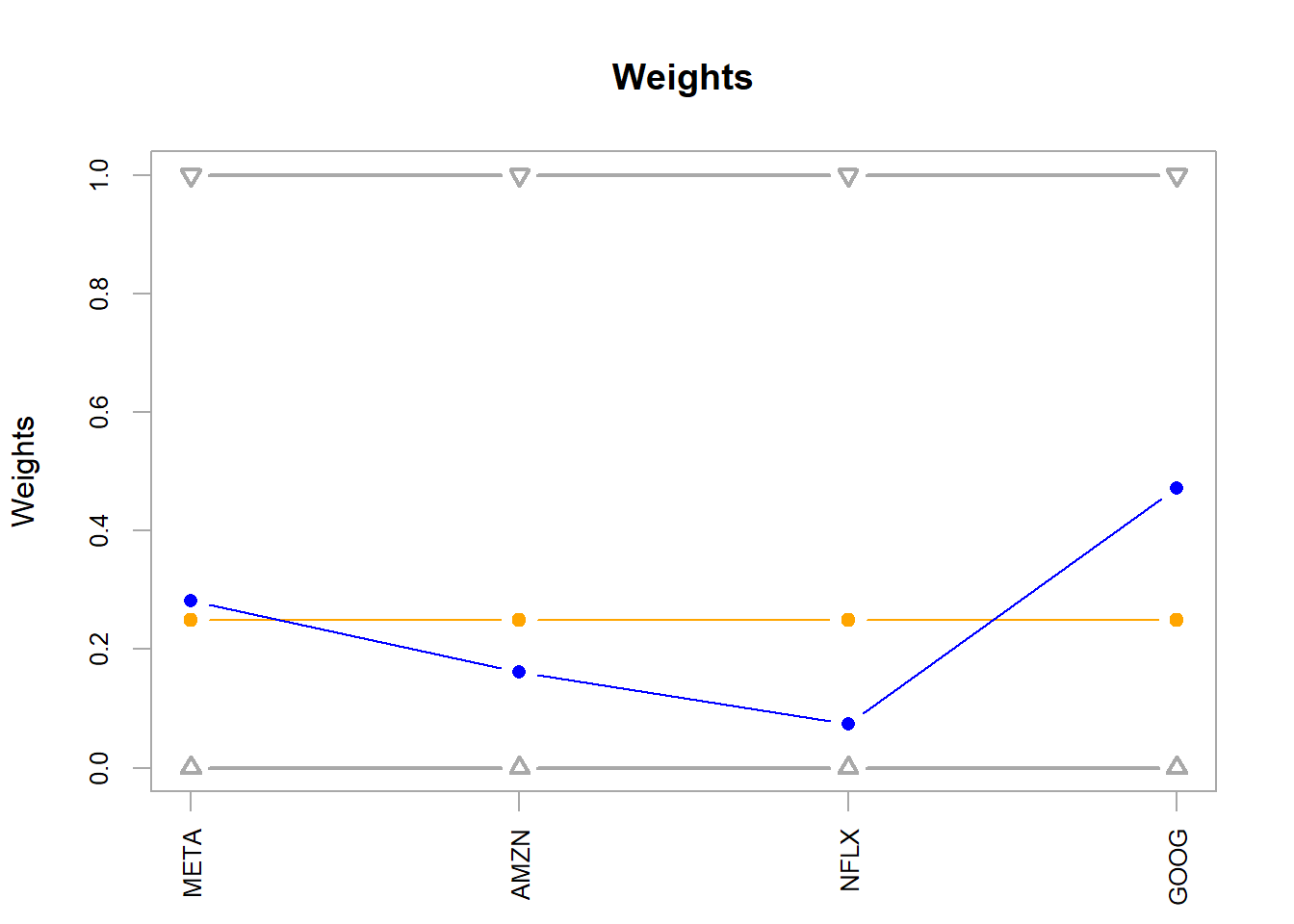
chart.Weights(opt_rand)
Figure 5.3: FANG, random method optimal weights.
The opt_rand weights define the implementable allocation.
# A tibble: 5 × 4
  symbol     mean     sd    sr
  <chr>     <dbl>  <dbl> <dbl>
1 opt_rand 0.0265 0.0581 0.456
2 NFLX     0.0592 0.167  0.355
3 META     0.0341 0.0989 0.345
4 AMZN     0.0257 0.0817 0.314
5 GOOG     0.0176 0.0594 0.296
The optimal portfolio opt_rand has a 0.4555797 return per unit of risk. Under this sample and criterion, it improves on the individual assets shown below.
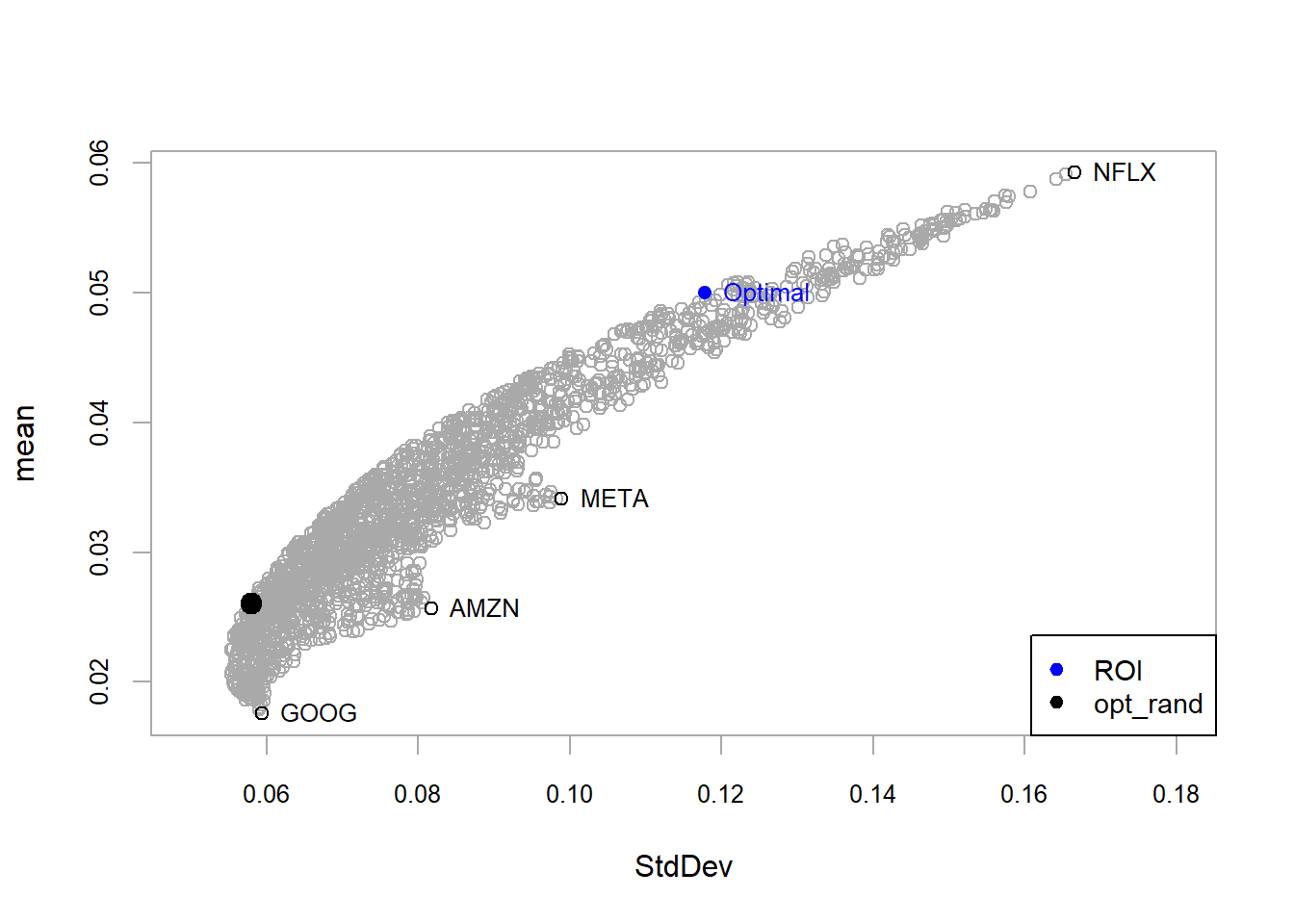
A second criterion is to optimize according to ROI (R Optimization Infrastructure for linear and quadratic programming solvers).
A different optimization method leads to a different portfolio. Both selected portfolios lie on the efficient frontier under the current data, constraints, and objective specification.
Code
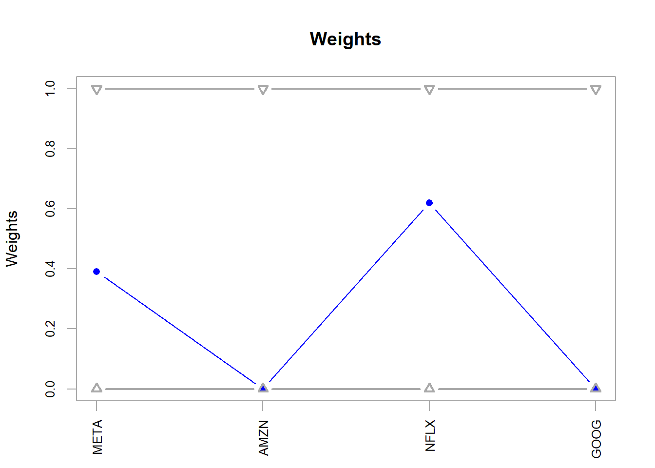
chart.Weights(opt_roi)
Figure 5.5: FANG, ROI method optimal weights.
The opt_roi weights define the allocation under the ROI method.
Code
extractWeights(opt_roi)
        META         AMZN         NFLX         GOOG
3.906783e-01 0.000000e+00 6.193217e-01 5.610126e-17
# A tibble: 6 × 4
  symbol     mean     sd    sr
  <chr>     <dbl>  <dbl> <dbl>
1 opt_rand 0.0265 0.0581 0.456
2 opt_roi  0.0500 0.118  0.424
3 NFLX     0.0592 0.167  0.355
4 META     0.0341 0.0989 0.345
5 AMZN     0.0257 0.0817 0.314
6 GOOG     0.0176 0.0594 0.296
The optimal portfolio opt_roi has a 0.4244362 return per unit of risk. The value exceeds the individual assets and remains below the opt_rand portfolio. According to this return-risk ratio, opt_rand ranks first in this comparison, with 0.4555797 return per unit of risk. The optimization process therefore produces a portfolio that improves on the individual assets in this historical sample. In practice, an allocation such as 28.2% in META, 16.2% in AMZN, 7.4% in NFLX, and 47.2% in GOOG would still require additional checks before implementation, including estimation stability, transaction costs, liquidity, constraints, and investor suitability.
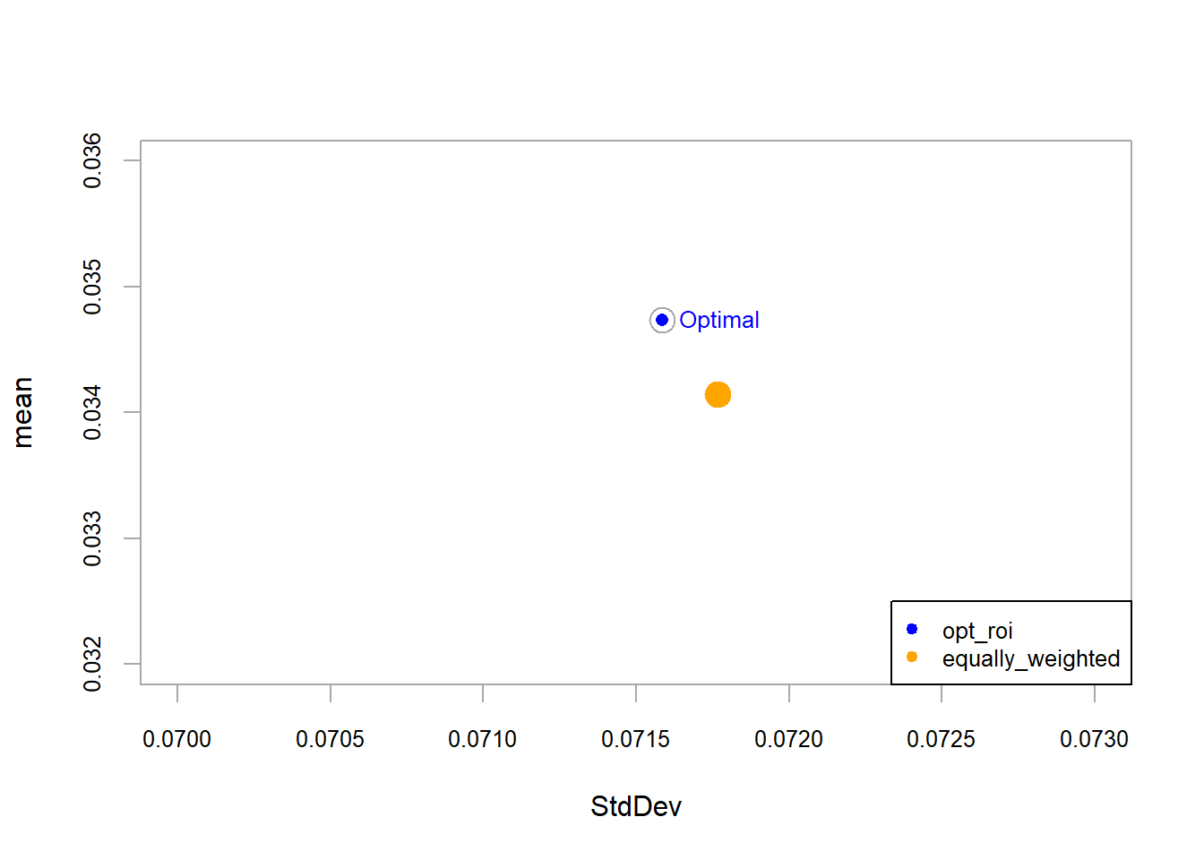
The orange portfolio represents an equally weighted benchmark with 25% in each asset. With \(N=4\), the weight is \(1/N=1/4\). This benchmark requires no optimization and still offers a diversified comparison point. In this example, it is close to the optimized alternatives and provides a useful check on whether optimization adds value under the selected assumptions.
A benchmark portfolio specification port_naive forces each weight to be exactly 0.25.
# A tibble: 7 × 4
  symbol      mean     sd    sr
  <chr>      <dbl>  <dbl> <dbl>
1 opt_naive 0.0341 0.0718 0.476
2 opt_rand  0.0265 0.0581 0.456
3 opt_roi   0.0500 0.118  0.424
4 NFLX      0.0592 0.167  0.355
5 META      0.0341 0.0989 0.345
6 AMZN      0.0257 0.0817 0.314
7 GOOG      0.0176 0.0594 0.296
The benchmark portfolio port_naive has the highest Sharpe ratio in this comparison, including the optimized alternatives. This result is informative: optimization depends on the objective, constraints, method, and sample estimates. A target-return constraint can search for an optimized portfolio that matches the benchmark portfolio’s expected return.
The expected return in \(t=0\) of the opt_rand portfolio is read from the optimizer output. It is the sum of the opt_rand portfolio weights multiplied by the individual expected returns. The realized return at \(t=1\) remains uncertain, so a simple simulation illustrates possible outcomes.
In this case, \(t=0\) is 2016-12-30 and \(t=1\) is 2017-01-31. The simulation uses the historical mean and standard deviation information available at \(t=0\).
The simulation generates 1,000 observations for each individual asset and portfolio. This simulation is a simple teaching device. It treats each investment alternative as normally distributed using the historical mean and standard deviation shown above.
It ignores time dependence, changing volatility, tail events, and the full correlation structure. The result is useful for intuition and works as a simplified risk model.
Code
# Number of simulations.sim =1000set.seed (7)# Simulation per stock and portfolio.s_AMZN <-rnorm(sim, 0.02566966, 0.08172605)s_FB <-rnorm(sim, 0.03412852, 0.09894324)s_GOOG <-rnorm(sim, 0.01757620, 0.05941703)s_NFLX <-rnorm(sim, 0.05919893, 0.16656346)s_ran <-rnorm(sim, opt_rand$opt_values$mean, opt_rand$opt_values$StdDev)s_roi <-rnorm(sim, opt_roi$opt_values$mean, opt_roi$opt_values$StdDev)
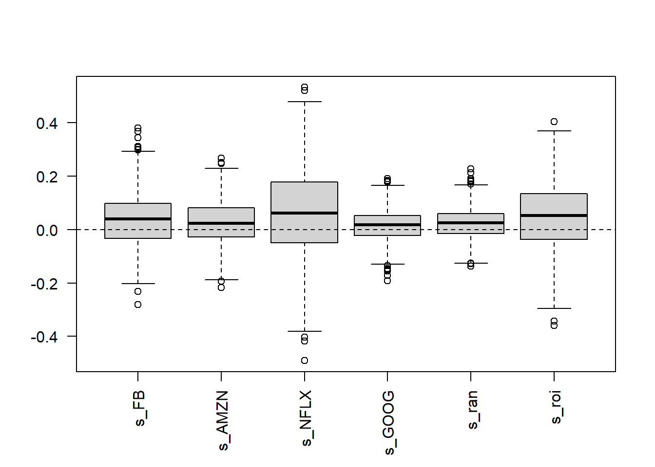
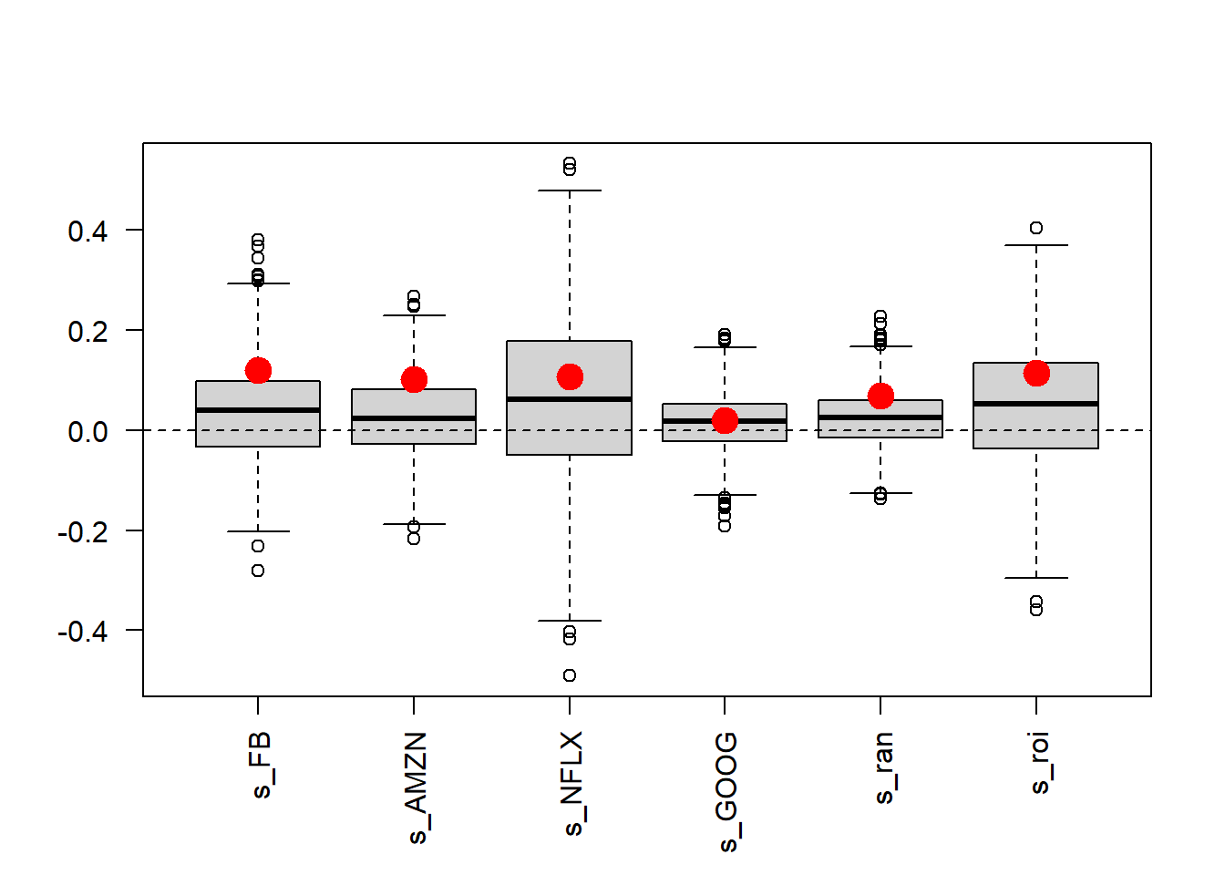
The simulated outcomes are summarized with a boxplot showing the minimum, maximum, median, first quartile, and third quartile.
Code
# The boxplot.b =cbind(s_FB, s_AMZN, s_NFLX, s_GOOG, s_ran, s_roi)boxplot(b, las =2)abline(h =0, lty =2)
Figure 5.8: FANG, simulated returns of investment alternatives.
The opt_rand portfolio has a narrower simulated dispersion than several individual stocks, while opt_roi has a wider simulated dispersion. Real returns can have heavier tails, changing volatility, and co-movement across assets, so this simulation works as a first approximation. Because the historical period is known, the realized returns on 2017-01-31 can be compared with the simulated distribution.
The 2017-01-31 realized returns provide the out-of-sample check. The FANG database ends at 2016-12-30, and these historical returns are fixed observations. They are stored directly here to avoid depending on the Meta ticker change or on current data-provider availability for old symbols.
      META       AMZN       NFLX       GOOG
0.12082830 0.10178200 0.10769470 0.02058163
These are the realized monthly returns at \(t=1\). They were unavailable when the portfolios were formed at \(t=0\), so they provide an out-of-sample check. The realized portfolio return is calculated as the weighted sum of realized individual returns.
The expected monthly return at \(t=0\) for the opt_rand portfolio is 0.02606294, and its realized monthly return at \(t=1\) is 0.06958923. For the opt_roi portfolio, the expected monthly return at \(t=0\) is 0.04999645, and the realized monthly return at \(t=1\) is 0.11390269. In this historical check, both realized returns exceeded their estimated values.
The plot below combines the simulated distribution with the realized returns shown in red.
Code
# The simulation.boxplot(b, las =2)abline(h =0, lty =2)# The realized returns in red.points(1, 0.1208283, col ="red", pch =19, cex =2)points(2, 0.101782, col ="red", pch =19, cex =2)points(3, 0.1076947, col ="red", pch =19, cex =2)points(4, 0.02058163, col ="red", pch =19, cex =2)points(5, sum(opt_rand$weights * r_stocks), col ="red",pch =19, cex =2)points(6, sum(opt_roi$weights * r_stocks), col ="red",pch =19, cex =2)
Figure 5.9: FANG, simulated returns of investment alternatives with realized returns in red.
The realized returns can be quite different from the simulated or expected returns. This difference depends on the method, the model, the sample length, the portfolio design, and the random component of returns. Portfolio models produce estimates under assumptions; realized returns can land far away from those estimates. In this FANG example, the optimized allocations performed well in the realized month.
The same allocation workflow is applied to the 10-stock data used in the previous asset-pricing example. The value of reproducible code is practical because once the data structure is consistent, the same modeling sequence can be reused with a different asset universe. The set keeps the same broad sector logic used before, where VTR represents healthcare real estate exposure and VOD represents telecommunications exposure.
# A tibble: 692 × 3
# Groups:   symbol [10]
   symbol date       R_stocks
   <chr>  <date>        <dbl>
 1 NEM    2010-01-29  -0.115
 2 NEM    2010-02-26   0.150
 3 NEM    2010-03-31   0.0355
 4 NEM    2010-04-30   0.101
 5 NEM    2010-05-28  -0.0403
 6 NEM    2010-06-30   0.149
 7 NEM    2010-07-30  -0.0946
 8 NEM    2010-08-31   0.0970
 9 NEM    2010-09-30   0.0268
10 NEM    2010-10-29  -0.0310
# ℹ 682 more rows
The portfolio specification uses the 10-asset return matrix.
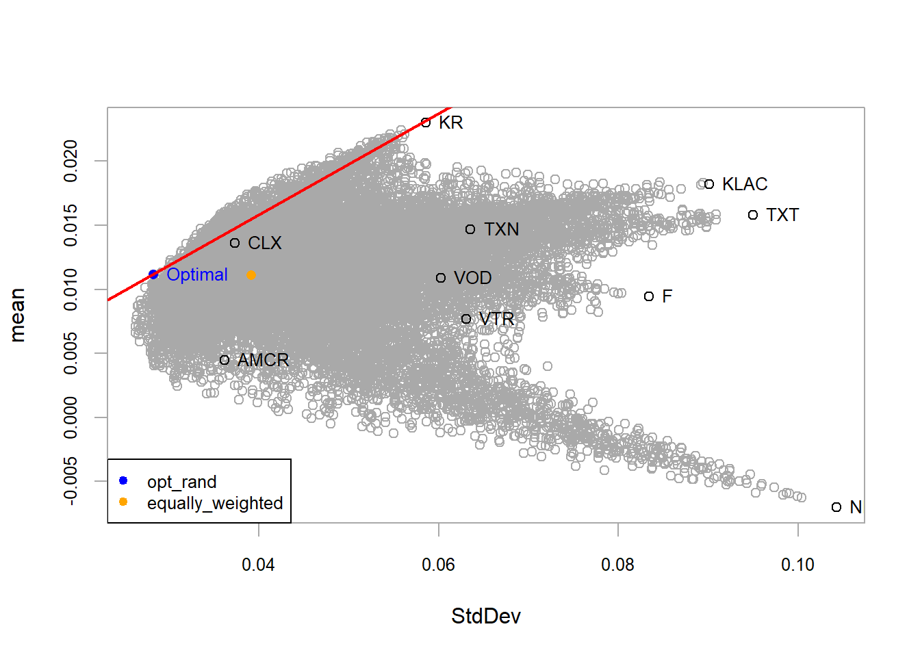
Figure 5.10: 10-assets, random method optimal portfolio.
Here, the slope of the red line corresponds to the optimal portfolio return per unit of risk. The optimal portfolio has a similar return per unit of risk to KR, while the rest of the assets have lower return per unit of risk in this sample.
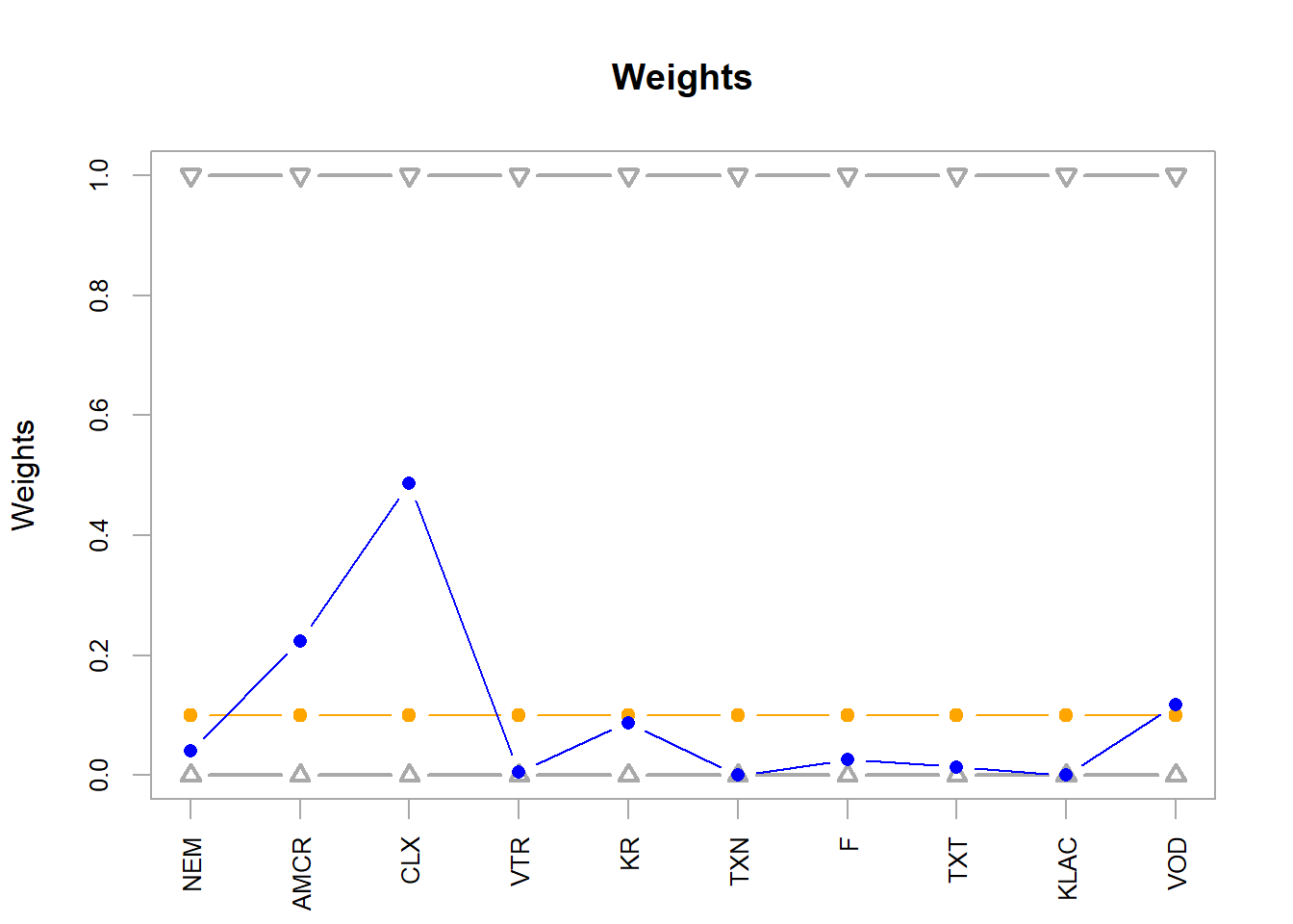
Code
extractWeights(opt_rand)
  NEM  AMCR   CLX   VTR    KR   TXN     F   TXT  KLAC   VOD
0.040 0.224 0.486 0.006 0.088 0.000 0.026 0.014 0.000 0.118
Code
chart.Weights(opt_rand)
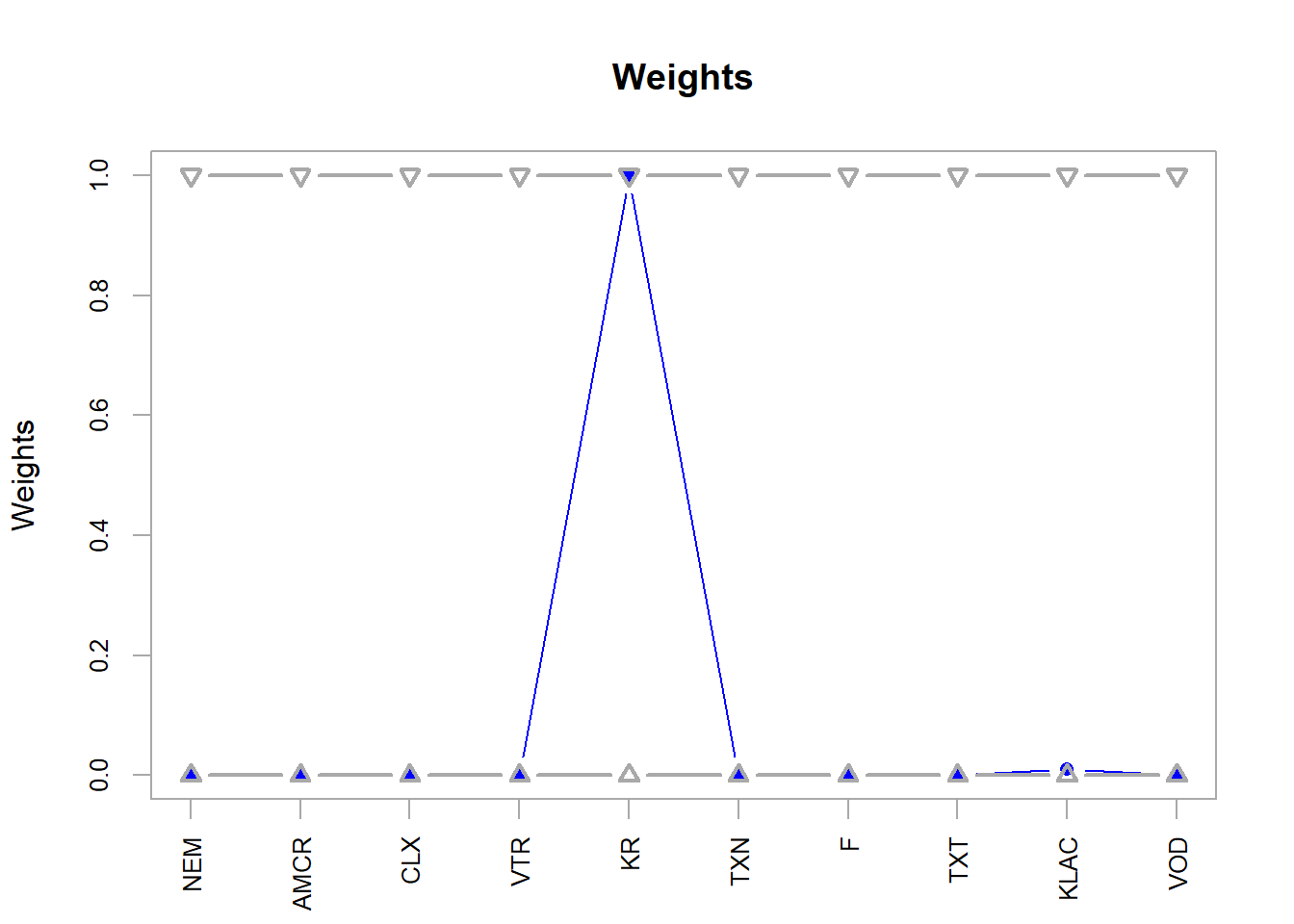
Figure 5.11: 10-assets, random method optimal weights.
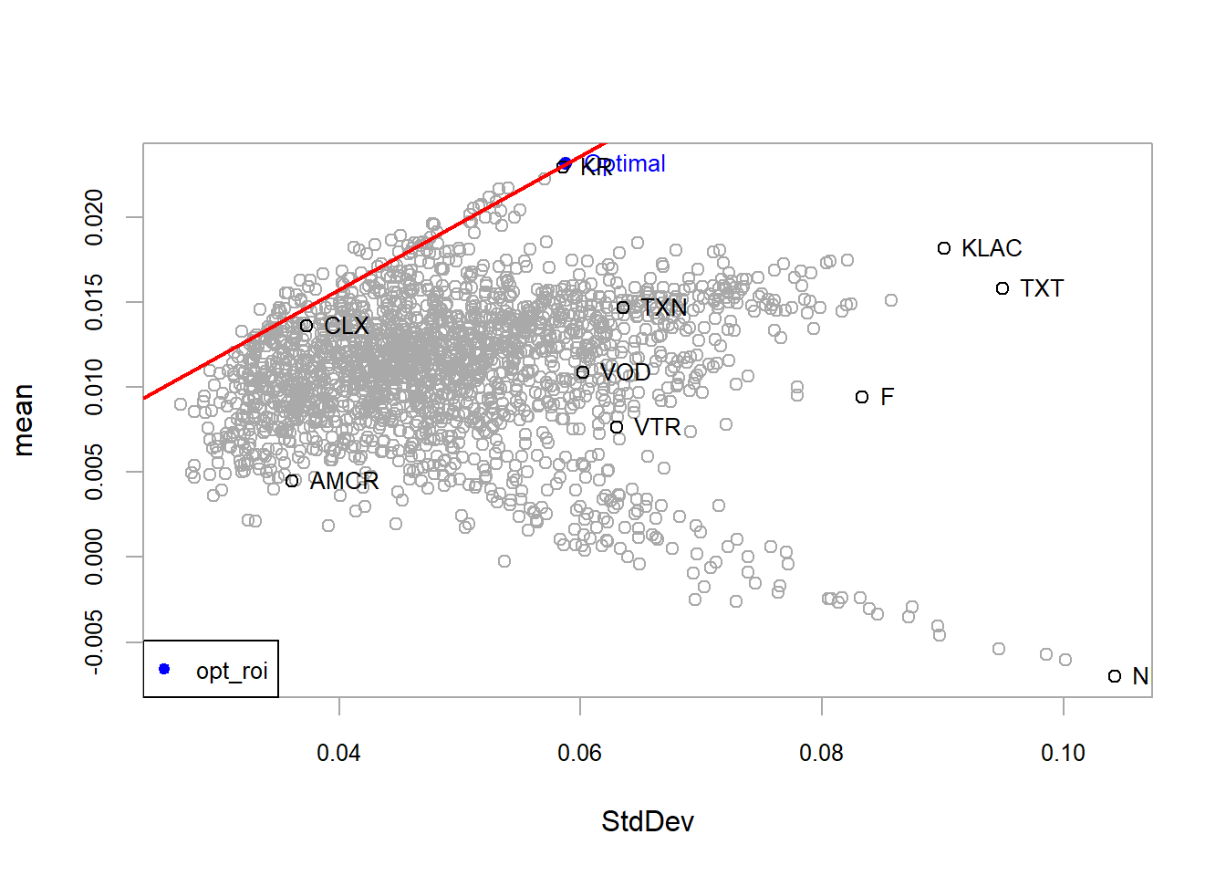
The ROI method provides a second optimization comparison for the same 10 assets.
Figure 5.12: 10-assets, ROI method optimal portfolio.
This solution is concentrated in KR, with a very small KLAC weight caused by the full-investment tolerance.
Code
extractWeights(opt_roi)
          NEM          AMCR           CLX           VTR            KR
 6.050516e-17  2.445685e-16  1.464562e-18  1.728497e-16  1.000000e+00
          TXN             F           TXT          KLAC           VOD
-9.142772e-17 -3.352468e-17  0.000000e+00  1.000000e-02  3.972525e-18
Code
chart.Weights(opt_roi)
Figure 5.13: 10-assets, ROI method optimal weights.
5.2 Diversification
In finance, diversification is the process of allocating capital in a way that reduces exposure to any single asset or risk factor. Holding several assets can reduce portfolio risk when their returns are imperfectly correlated. If the assets move almost together, as Visa and Mastercard did in the previous chapter, diversification gains are limited. This section uses a controlled experiment: two artificial assets, \(X\) and \(Y\), are added to the FANG database to create a six-asset universe. Their strong negative correlation isolates the mechanism through which diversification can reduce portfolio volatility.
The returns of the two new assets are simulated. The assets \(X\) and \(Y\) do not exist in the real world; they are created to isolate the diversification mechanism.
Code
set.seed(13)data =mvrnorm(n =48, mu =c(0.2, 0.5),Sigma =matrix(c(1, -1.4, -1.4, 2), nrow =2),empirical =TRUE)/10xy =as.data.frame(data)X = xy$V1Y = xy$V2# Add X and Y to the fang database.fang_xy <- fangfang_xy$X <- Xfang_xy$Y <- Yhead(fang_xy)
The correlation matrix verifies that the two new assets are negatively correlated.
Code
cor(fang_xy)
            META        AMZN        NFLX       GOOG           X           Y
META  1.00000000  0.18461970  0.21820791  0.2468989  0.03779375 -0.04276241
AMZN  0.18461970  1.00000000  0.31180203  0.6171376  0.04877402 -0.05611269
NFLX  0.21820791  0.31180203  1.00000000  0.3586214  0.06772682 -0.05943567
GOOG  0.24689886  0.61713764  0.35862138  1.0000000  0.20682201 -0.19110508
X     0.03779375  0.04877402  0.06772682  0.2068220  1.00000000 -0.98994949
Y    -0.04276241 -0.05611269 -0.05943567 -0.1911051 -0.98994949  1.00000000
The correlation of \(X\) and \(Y\) is -0.98994949, very close to -1, so they are strongly negatively correlated. Their correlations with the original assets are also negative. Under the same objective, this expanded universe creates room for a portfolio with a stronger return per unit of risk.
Negative correlation reduces the covariance component of portfolio variance. Expected return is still the weighted average of the individual expected returns, so it does not mechanically become zero.
A sequence of \(X\) and \(Y\) portfolio weights is created.
Code
w_x <-seq(0, 1, 0.01)w_y <-1- w_x
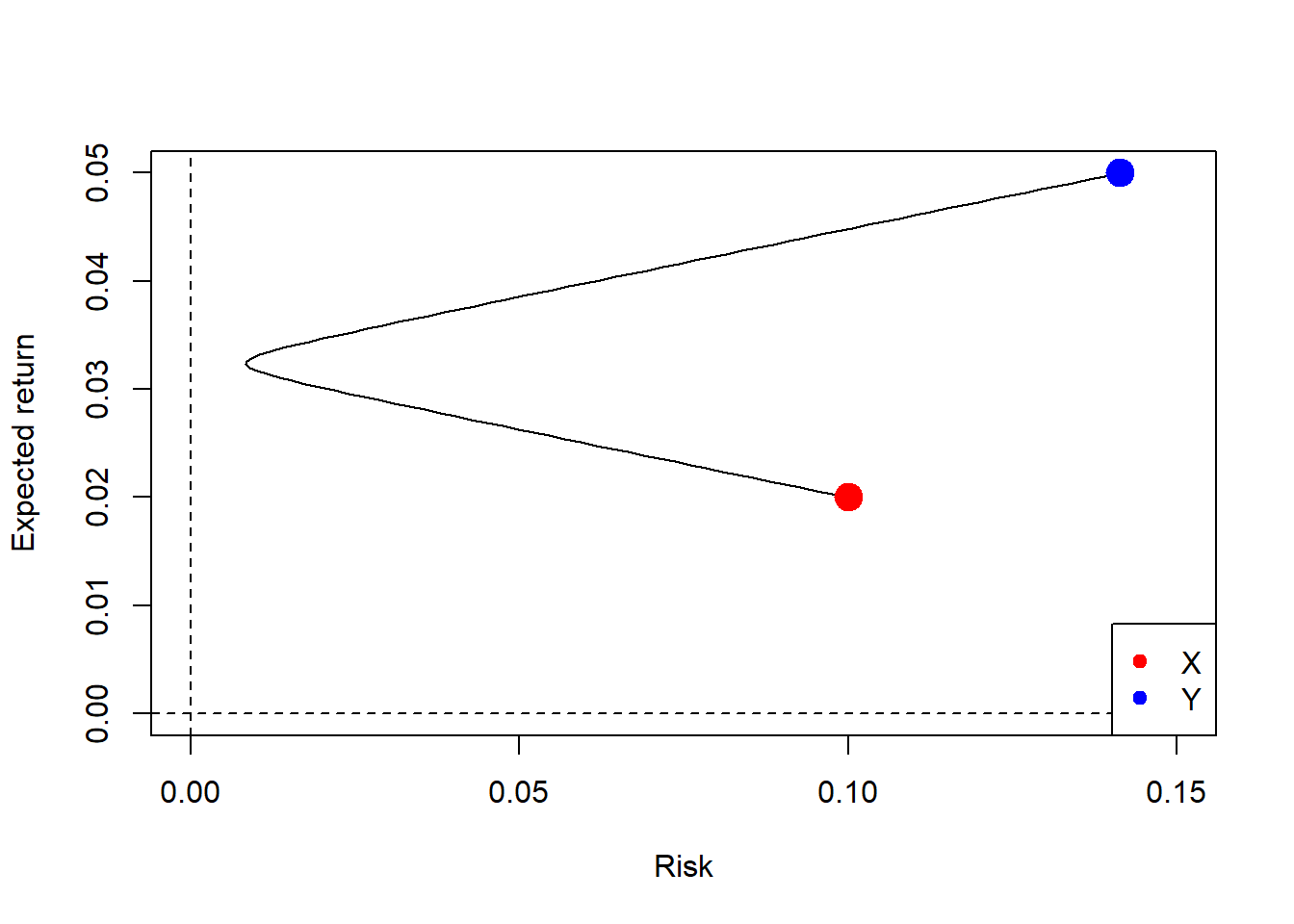
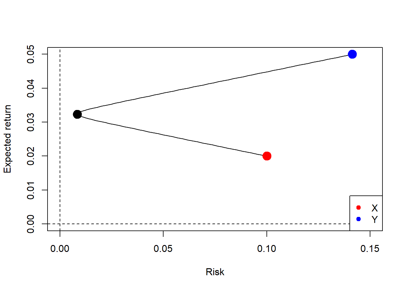
For a two-asset portfolio, expected return remains a weighted average and risk depends on variances plus covariance.
Figure 5.15: 2-assets, efficient frontier and minimum variance portfolio.
The minimum-variance portfolio weights are shown below.
Code
w_x[60]
[1] 0.59
Code
w_y[60]
[1] 0.41
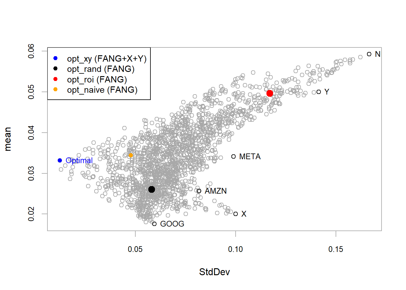
The FANG database is then combined with the two artificial assets \(X\) and \(Y\). The portfolio specification and optimization are rebuilt with this expanded asset universe.
The new assets materially change the optimization because their negative correlation creates a diversification opportunity. The optimal portfolio has almost the same expected return as Meta with substantially lower risk. Correlation therefore plays a central role in diversification: assets with low or negative correlation can reduce portfolio volatility when combined with the rest of the investment universe.
The details of the new portfolio show how the optimizer uses the artificial diversification opportunity.
Code
# Extract weight, risk and return.extractWeights(opt_xy)
 META  AMZN  NFLX  GOOG     X     Y
0.002 0.028 0.000 0.014 0.522 0.434
The portfolio assigns high weights to \(X\) and \(Y\), with values of 52.2% and 43.4%. The rest is 0.2% in META, 2.8% in AMZN, 0% in NFLX, and 1.4% in GOOG.
The opt_xy portfolio shows a large improvement because the artificial assets combine high average returns with a very strong negative correlation. This controlled experiment isolates the diversification mechanism. In practice, investors evaluate return together with volatility, correlation, liquidity, estimation error, and implementation constraints. Low or negatively correlated assets can reduce portfolio volatility and improve the return per unit of risk, while realized returns remain uncertain.
A practical extension is to search for assets with different exposures to risk factors, estimate their joint behavior, and rerun the optimization with realistic constraints. Sector, geography, currency, liquidity, and macroeconomic exposure are natural places to start that search.
5.3 Portfolio rebalancing and evaluation
The previous sections estimate portfolio weights once. The optimization criterion changed and new assets were added, while the allocation was still selected at a single point in time. Rebalancing extends the problem by recalculating portfolio weights as new returns become available. Evaluation then asks how the resulting strategy performs over a full investment period. This section incorporates both ideas with a different database.
Consider the following investment process. At \(t=0\), the investor has access to 60 months of historical information for a set of individual assets. The data from \(t=-60\) to \(t=0\) is used to estimate portfolio weights and form the portfolio at \(t=0\). Returns are then realized for \(t=1\), \(t=2\), and \(t=3\). At \(t=3\), the portfolio is re-estimated using the rolling window from \(t=-57\) to \(t=3\). The same procedure continues through the investment period. The evaluation question is whether the rebalanced strategy produces stronger annualized return and return per unit of risk than a benchmark.
The process requires repeated data transformation, optimization, implementation, and evaluation. R makes the workflow reproducible because each rebalance date follows the same script. That automation is important in finance: the analyst can focus on assumptions, constraints, risk controls, and interpretation while the computer performs the repeated calculations.
The rebalancing exercise starts with the asset-return data.
Code
# Get the data.data(indexes)returns <- indexes[, 1:4]tail(returns)
The database goes from 1980-01-31 to 2009-12-31. The assets are US Bonds, US Equities, International Equities, and Commodities. The first allocation is calculated with the initial 60 monthly observations, and later allocations are updated according to the quarterly rebalancing schedule. The realized evaluation period starts after the training window and ends on 2009-12-31.
Before calculating optimal portfolios, a benchmark portfolio is created. This allows the optimized portfolio to be compared with a simple alternative. In this case, the benchmark is an equally weighted portfolio, investing 25% in each asset for all periods. With \(N=4\) assets
\[
w_i=\frac{1}{4}=0.25.
\]
This equally weighted portfolio requires no optimization. It invests 25% in each asset, or index in this case, and keeps that benchmark rule through the investment period.
The benchmark gives the optimized strategy a simple comparison point.
The portfolio specification follows the same structure used in the previous section.
Code
# Base portfolio specification.base_port_spec <-portfolio.spec(assets =colnames(returns))#base_port_spec <- add.constraint(portfolio = base_port_spec,# type = "full_investment")#base_port_spec <- add.constraint(portfolio = base_port_spec,# type = "long_only")base_port_spec <-add.constraint(portfolio = base_port_spec,type ="weight_sum",min_sum =0.99, max_sum =1.01)base_port_spec <-add.constraint(portfolio = base_port_spec,type ="box", min =0, max =1)base_port_spec <-add.objective(portfolio = base_port_spec,type ="risk", name ="StdDev")
The investment process is implemented with quarterly rebalancing. At each rebalance date, the portfolio return for the next period is determined by the weights chosen from the prior information set.
\[
R_{p,t}=\sum_{i=1}^{N}w_{i,t-1}R_{i,t}.
\]
Code
# Run the optimization with periodic rebalancing.opt_base <-optimize.portfolio.rebalancing(R = returns,optimize_method ="ROI", portfolio = base_port_spec,rebalance_on ="quarters", training_period =60,rolling_window =60)# Calculate portfolio returns.base_returns <-Return.portfolio(returns, extractWeights(opt_base))colnames(base_returns) <-"base"
The rebalancing and evaluation calculations are complete, so the allocation path can be inspected.
Code
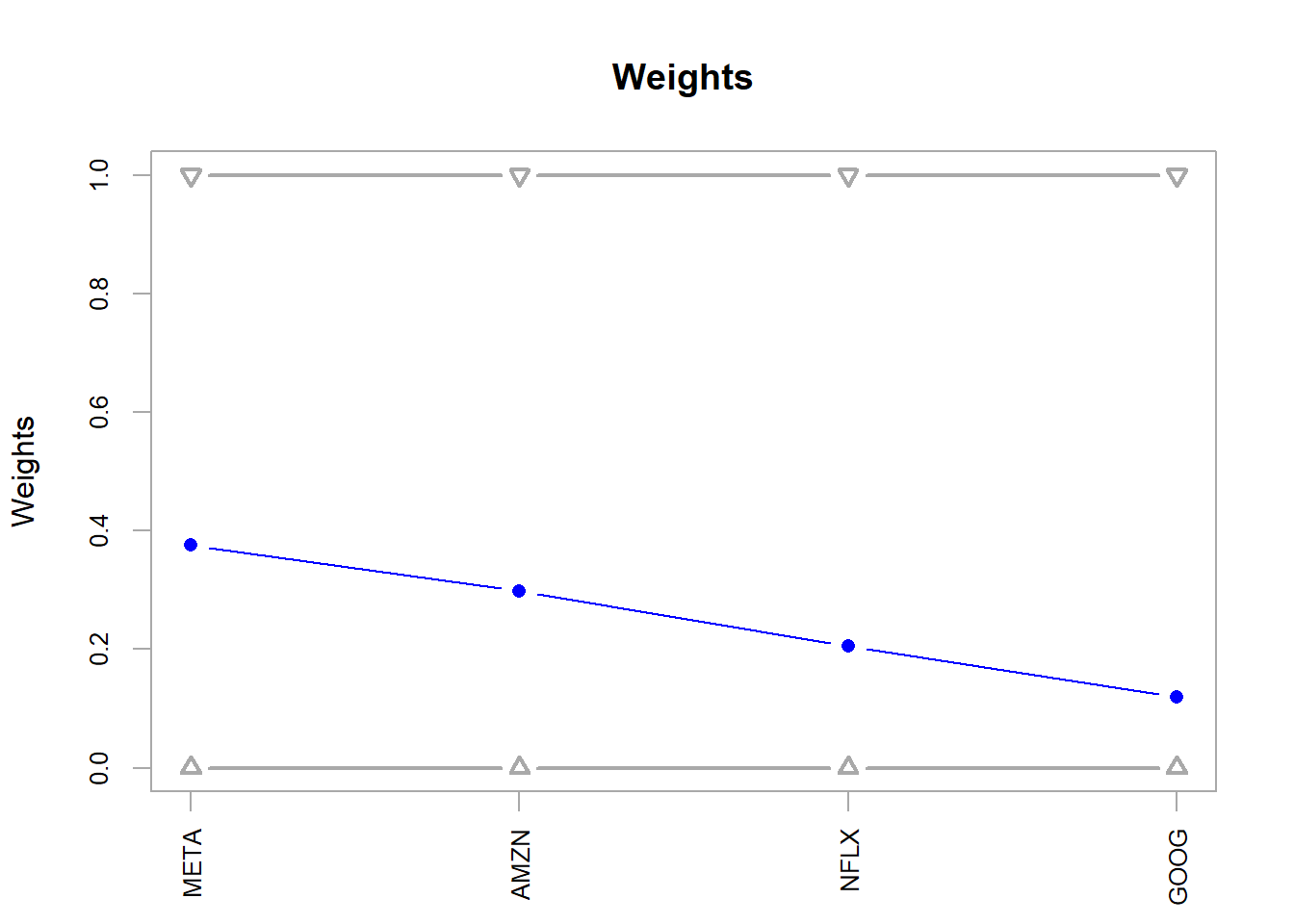
# Chart the optimal weights.chart.Weights(opt_base)
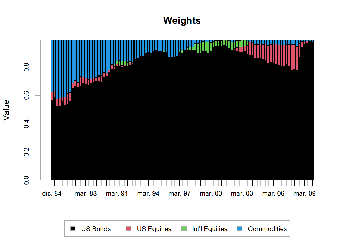
Figure 5.17: Indexes, optimal weights.
The chart shows the weight assigned to each asset through the rebalancing process. US bonds dominate the allocation in this run, which reflects the optimization objective and historical inputs. The annualized performance table reports the realized backtest comparison.
Code
# Merge benchmark and portfolio returns.ret <-cbind(benchmark_returns, base_returns)# Annualized performance.table.AnnualizedReturns(ret)
                          benchmark   base
Annualized Return            0.0769 0.0765
Annualized Std Dev           0.1029 0.0432
Annualized Sharpe (Rf=0%)    0.7476 1.7710
The optimized strategy produced a higher annualized return than the benchmark in this historical backtest. As a sample result, it is read together with the assumptions, constraints, and historical window used to generate it.
Investment mandates often impose limits on individual assets. Suppose the portfolio is not allowed to invest more than 40% in US bonds. This constraint can be incorporated directly before rerunning the rebalancing exercise.
Code
# Make a copy of the portfolio specification.box_port_spec <- base_port_spec# Update the constraint.box_port_spec <-add.constraint(portfolio = box_port_spec,type ="box", min =0.05, max =0.4,indexnum =2)# Backtest.opt_box <-optimize.portfolio.rebalancing(R = returns,optimize_method ="ROI",portfolio = box_port_spec,rebalance_on ="quarters",training_period =60,rolling_window =60)# Calculate portfolio returns.box_returns <-Return.portfolio(returns, extractWeights(opt_box))colnames(box_returns) <-"box"
Additional constraints reduce the feasible set available to the optimizer. They may be necessary for mandate, liquidity, or risk-control reasons, although they can reduce performance under the selected objective.
Code
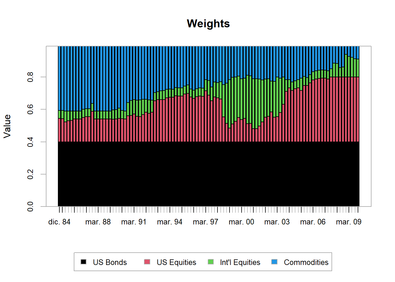
# Chart the optimal weights.chart.Weights(opt_box)
Indexes, optimal weights with box constraint.
The constraint forces the allocation to spread more weight across the remaining assets.
                          benchmark   base    box
Annualized Return            0.0769 0.0765 0.0753
Annualized Std Dev           0.1029 0.0432 0.0806
Annualized Sharpe (Rf=0%)    0.7476 1.7710 0.9344
In this backtest, the box constraint reduces the annualized return relative to the unconstrained optimized strategy.
Private firms often provide recurring portfolio analysis, monitoring, and rebalancing services. Software has reduced the cost of producing this kind of analysis, and fintech firms can now offer tools that were previously available only to institutions with specialized teams and infrastructure. Even so, functions such as optimize.portfolio() are professional modeling tools. They support the decision process, while the final portfolio decision still requires data validation, risk controls, costs, constraints, and suitability analysis.
Code
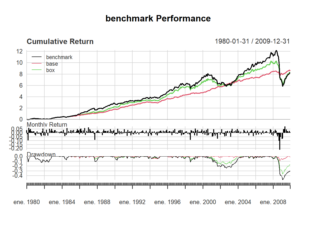
charts.PerformanceSummary(R = ret)
Figure 5.18: Indexes, portfolio performance.
Portfolio allocation produces weights, realized returns, and benchmark comparisons. The following chapter expresses the same portfolio problem in terms of possible losses. Value at Risk provides a compact way to ask how large a one-day portfolio loss could be under a chosen confidence level and a specific modeling assumption.