6 Value at Risk
The previous chapter focused on how to allocate capital across assets. The complementary risk-management task is to estimate how large a short-run market loss could be once a portfolio exists. Value at Risk (VaR) provides a compact answer by combining a time horizon, a confidence level, portfolio weights, and a loss distribution.
If \(L\) is the portfolio loss over the chosen horizon and \(\alpha\) is the confidence level, VaR is the loss threshold such that losses are below or equal to it with probability \(\alpha\).
\[ P(L \leq VaR_\alpha)=\alpha. \]
Equivalently, when losses are sorted from low to high, VaR is the corresponding loss quantile.
\[ VaR_\alpha = Q_\alpha(L), \]
where \(Q_\alpha(L)\) is the \(\alpha\) quantile of the loss distribution.
This chapter develops and extends the example called Investment in Four Stock Indices in Chapters 22 and 23 of Hull (2015). In this book, the example is used as an integrative market-risk exercise within the broader Financial Modeling with R path. It combines several ideas already used in the book: data preparation, currency adjustment, returns, portfolio weights, optimization, scenario generation, quantiles, and realized-outcome evaluation. The database used in this example dataR.txt is available here.
The working question is specific: calculate VaR for a portfolio using a one-day time horizon, a 99% confidence level, and 501 days of data, from Monday August 7, 2006 to Thursday September 25, 2008. The chapter follows four steps: express all index positions in US dollars, build one-day loss scenarios, estimate VaR with historical and model-building methods, and evaluate how portfolio weights change the loss distribution.
6.1 Prepare the data
The data set contains the index levels and exchange rates needed to express all positions from the perspective of a US investor.
The first rows show the raw structure of the file before currency adjustment.
      DJIA FTSE100 USDGBP   CAC40 EURUSD   Nikkei YENUSD
1 11219.38  5828.8 1.9098 4956.34 0.7776 15154.06 115.00
2 11173.59  5818.1 1.9072 4967.95 0.7789 15464.66 115.08
3 11076.18  5860.5 1.9086 5025.15 0.7762 15656.59 115.17
4 11124.37  5823.4 1.8918 4976.64 0.7828 15630.91 115.41
5 11088.02  5820.1 1.8970 4985.52 0.7833 15565.02 116.07
6 11097.87  5870.9 1.8923 5046.93 0.7847 15857.11 116.45
These are four international stock indices: Dow Jones Industrial Average (DJIA) in the US, the FTSE 100 in the UK, the CAC 40 in France, and the Nikkei 225 in Japan together with the corresponding exchange rates.
Because the example uses the perspective of a US investor, the values of the FTSE 100, CAC 40, and Nikkei 225 must be measured in US dollars. The adjusted US dollar equivalents of the stock indices follow these conversions.
\(FTSE_{USD}=FTSE_{GBP}\times\frac{USD}{GBP}\).
\(CAC_{USD}=\frac{CAC_{EUR}}{\frac{EUR}{USD}}\).
\(Nikkei_{USD}=\frac{Nikkei_{JPY}}{\frac{JPY}{USD}}\).
The following table shows the US dollar equivalent of the stock indices used for historical simulation.
  Day     DJIA  AFTSE100   ACAC40  ANikkei
1   0 11219.38 11131.842 6373.894 131.7744
2   1 11173.59 11096.280 6378.162 134.3818
3   2 11076.18 11185.350 6474.040 135.9433
4   3 11124.37 11016.708 6357.486 135.4381
5 499 10825.17  9438.580 6033.935 114.2604
6 500 11022.06  9599.898 6200.396 112.8221
The VaR estimation uses 501 observations because the sample counts from day zero through day 500. The A before the index name stands for adjusted. The figure shows the common dollar-based scale that will be used for scenario construction.
Code
df.Adj %>%
  mutate(ANikkei = ANikkei*100) %>%
  mutate(obs = c(1:502)) %>%
  select(obs, DJIA, AFTSE100, ACAC40, ANikkei) %>%
  filter(obs < 502) %>%
  gather(IX, Adj, DJIA, AFTSE100, ACAC40, ANikkei) %>%
  mutate(IX = as.factor(IX)) %>%
  ggplot(aes(x = obs, y = Adj, col = IX)) +
  geom_line(size = 1) +
  labs(y = "US dollar equivalent of stock indices", x = "") +
  theme(legend.position = "bottom")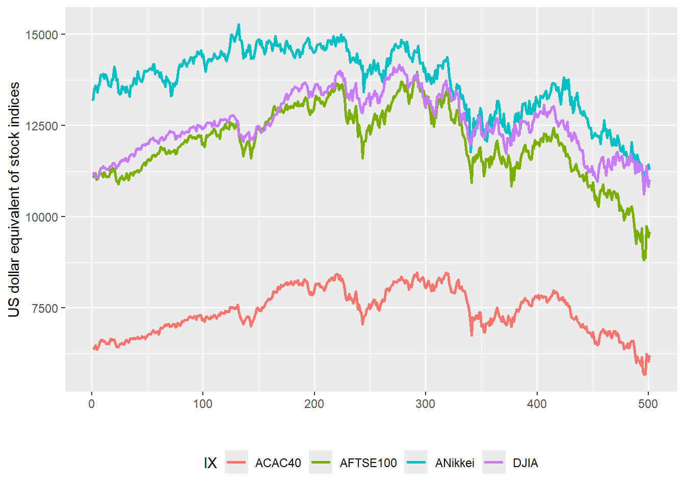
The time series starts on Monday August 7, 2006 and ends on Thursday September 25, 2008. These are 501 past daily observations. The plot below also shows the value of Friday September 26, 2008 as a dot. This is observation 502, stored as tomorrow. Observation 502 is excluded from the VaR estimation because it represents the future value being evaluated.
Code
tomorrow <- df.Adj %>%
  mutate(ANikkei = ANikkei*100) %>%
  mutate(obs = c(1:502)) %>%
  select(obs, DJIA, AFTSE100, ACAC40, ANikkei) %>%
  filter(obs == 502) %>%
  gather(IX, Adj, DJIA, AFTSE100, ACAC40, ANikkei) %>%
  mutate(IX = as.factor(IX))

df.Adj %>%
  mutate(ANikkei = ANikkei*100) %>%
  mutate(obs = c(1:502)) %>%
  select(obs, DJIA, AFTSE100, ACAC40, ANikkei) %>%
  filter(obs > 400) %>%
  filter(obs < 502) %>%
  gather(IX, Adj, DJIA, AFTSE100, ACAC40, ANikkei) %>%
  mutate(IX = as.factor(IX)) %>%
  ggplot(aes(x = obs, y = Adj, col = IX)) +
  geom_line(size = 1) +
  geom_point(aes(obs, Adj), size = 2, alpha = 0.4, data = tomorrow) +
  labs(y = "US dollar equivalent of stock indices", x = "") +
  theme(legend.position = "bottom")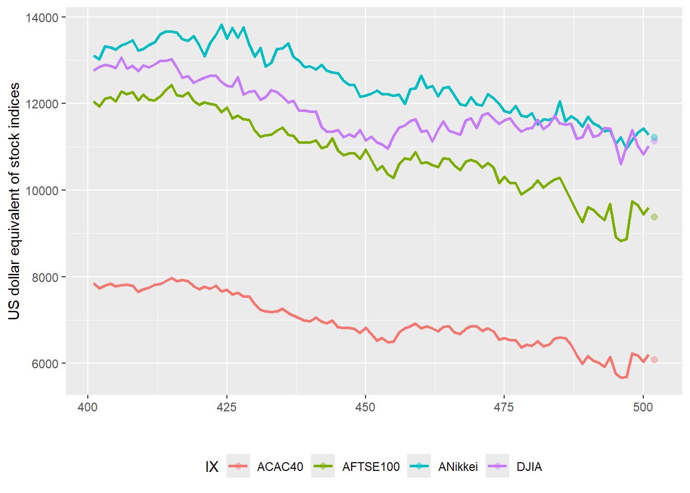
The stock index values for Friday September 26, 2008 provide the realized values used later for evaluation.
6.2 Historical simulation
The historical simulation method requires scenarios for the possible stock-index values on Friday September 26, 2008. The calculation constructs 500 scenarios from 501 past observations. The method assumes that the index value on Friday September 26, 2008 can be represented by the value observed on Thursday September 25, 2008 multiplied by one historical percentage change. The first percentage change goes from Monday August 7, 2006 to Tuesday August 8, 2006. The second goes from Tuesday August 8, 2006 to Wednesday August 9, 2006, and the sequence continues through the historical window.
For index \(j\) and historical scenario \(k\), the generated value is defined by applying a past daily relative change to the last observed value.
\[ S_{j,k}^{scenario}=S_{j,T}\frac{S_{j,k}}{S_{j,k-1}}, \qquad k=1,\dots,500. \]
The portfolio value and loss for scenario \(k\) combine those scenario index levels with the dollar allocations.
\[ p_k=\sum_{j=1}^{4} a_j \frac{S_{j,k}^{scenario}}{S_{j,T}}, \qquad l_k=10{,}000-p_k, \]
where \(a_j\) is the dollar allocation to index \(j\) in thousands of US dollars.
The adjusted values provide the reference levels for the scenario ratios.
  Day     DJIA  AFTSE100   ACAC40  ANikkei
1   0 11219.38 11131.842 6373.894 131.7744
2   1 11173.59 11096.280 6378.162 134.3818
3   2 11076.18 11185.350 6474.040 135.9433
4   3 11124.37 11016.708 6357.486 135.4381
5 499 10825.17  9438.580 6033.935 114.2604
6 500 11022.06  9599.898 6200.396 112.8221
The first three Dow Jones scenarios \(SDJIA\) illustrate the calculation.
\(SDJIA_1 = 11022.06 \times \frac{11173.59}{11219.38} \rightarrow SDJIA_1 = 10977.08\).
\(SDJIA_2 = 11022.06 \times \frac{11076.18}{11173.59} \rightarrow SDJIA_2 = 10925.97\)
\(SDJIA_3 = 11022.06 \times \frac{11124.37}{11076.18} \rightarrow SDJIA_3 = 11070.01\)
The first three possible Dow Jones values according to the historical approach for September 26, 2008 are 10977.08, 10925.97, and 11070.01. The actual value, 11143.130, is reserved for evaluation, so it does not enter the VaR estimate.
The generated scenario table gives the first simulated values and the last historical rows in the scenario window.
Code
df.Adj.S <- df.Adj %>%
  mutate(obs = c(0:501)) %>%
  mutate(SDJIA = DJIA[501] * (DJIA/lag(DJIA))) %>%
  mutate(SFTSE100 = AFTSE100[501] * (AFTSE100/lag(AFTSE100))) %>%
  mutate(SCAC40 = ACAC40[501] * (ACAC40/lag(ACAC40))) %>%
  mutate(SNikkei = ANikkei[501] * (ANikkei/lag(ANikkei)))

df.Adj.S %>%
  select(obs, SDJIA, SFTSE100, SCAC40, SNikkei) %>%
  slice(2, 3, 4, 500, 501)
obs SDJIA SFTSE100 SCAC40 SNikkei
1 1 10977.08 9569.230 6204.547 115.0545
2 2 10925.97 9676.957 6293.603 114.1331
3 3 11070.01 9455.160 6088.768 112.4028
4 499 10831.43 9383.488 6051.936 113.8498
5 500 11222.53 9763.974 6371.450 111.4019The violin plot shows the generated scenarios together with the actual values for September 26, 2008. The dot is useful for evaluation because it shows where the realized next-day value landed relative to the historical scenario range.
Code
levels(tomorrow$IX) <- list(SCAC40 = "ACAC40", SDJIA = "DJIA",
                         SFTSE100 = "AFTSE100", SNikkei = "ANikkei")

df.Adj.S %>%
  mutate(SNikkei = SNikkei*100) %>%
  mutate(obs = c(1:502)) %>%
  select(obs, SDJIA, SFTSE100, SCAC40, SNikkei) %>%
  filter(obs < 502) %>%
  gather(IX, S, SDJIA, SFTSE100, SCAC40, SNikkei) %>%
  mutate(IX = as.factor(IX)) %>%
  ggplot(aes(x = IX, fill = IX)) +
  geom_violin(aes(IX, S), draw_quantiles = 0.5) +
  geom_point(aes(IX, Adj), size = 3,
             data = tomorrow, show.legend = FALSE) +
  labs(y = "Scenarios generated for September 26, 2008", x = "") +
  theme(legend.position = "none")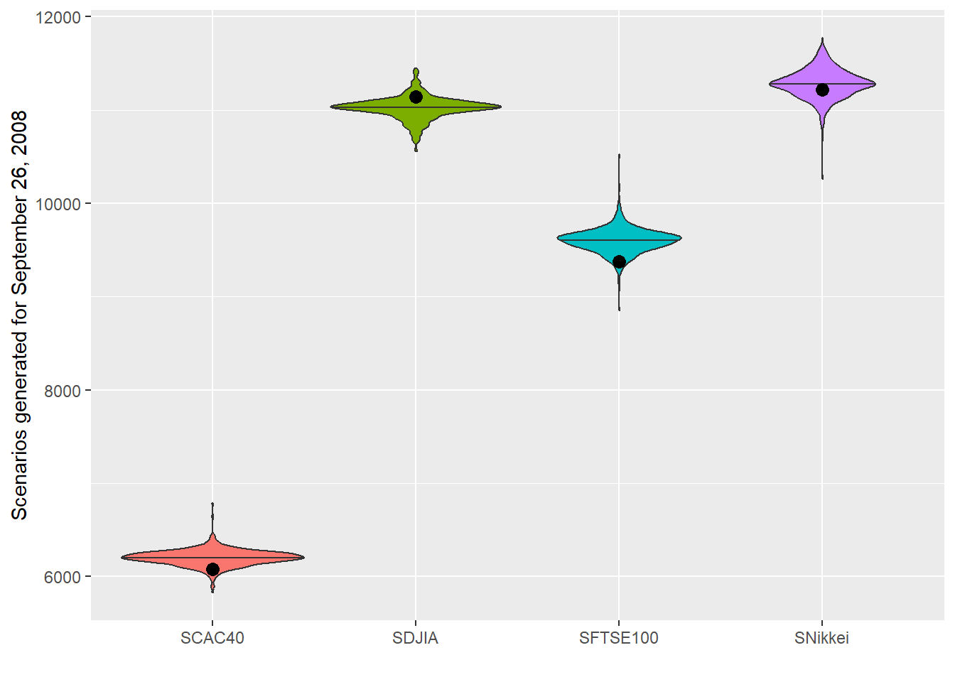
According to the example, an investor in the United States owns, on September 25, 2008, a portfolio worth $10 million consisting of 40% in the DJIA, 30% in the FTSE, 10% in the CAC, and 20% in the Nikkei. The calculations below express portfolio values and losses in thousands of US dollars. The corresponding 500 scenarios for the possible portfolio value \(p\) on September 26, 2008 use the same allocation formula.
\(p_1 = 4000 \frac{SDJIA_1}{DJIA_{sept.25.2008}} + 3000 \frac{SFTSE_1}{FTSE_{sept.25.2008}} + 1000 \frac{SCAC_1}{CAC_{sept.25.2008}} + 2000 \frac{SNikkei_1}{Nikkei_{sept.25.2008}}\),
\(p_1 = 4000 \frac{10977.08}{11022.06} + 3000 \frac{9569.230}{9599.898} + 1000 \frac{6204.547}{6200.396} + 2000 \frac{115.0545}{112.8221}\),
\(p_1 = 10{,}014.334\) thousand dollars.
\(p_2 = 4000 \frac{SDJIA_2}{DJIA_{sept.25.2008}} + 3000 \frac{SFTSE_2}{FTSE_{sept.25.2008}} + 1000 \frac{SCAC_2}{CAC_{sept.25.2008}} + 2000 \frac{SNikkei_2}{Nikkei_{sept.25.2008}}\),
\(p_2 = 4000 \frac{10925.97}{11022.06} + 3000 \frac{9676.957}{9599.898} + 1000 \frac{6293.603}{6200.396} + 2000 \frac{114.1331}{112.8221}\),
\(p_2 = 10{,}027.481\) thousand dollars.
The same scenario formula is applied to the remaining historical changes.
Code
df.Adj.S <- df.Adj.S %>%
  mutate(p = (4000 * SDJIA / DJIA[501]) + # Investment portfolio value
             (3000 * SFTSE100 / AFTSE100[501]) +
             (1000 * SCAC40 / ACAC40[501]) +
             (2000 * SNikkei / ANikkei[501])) %>%
  mutate(l = 10000 - p) # Losses l

df.Adj.S %>%
  select(obs, SDJIA, SFTSE100, SCAC40, SNikkei, p, l) %>%
  slice(2, 3, 4, 500, 501)
obs SDJIA SFTSE100 SCAC40 SNikkei p l
1 1 10977.08 9569.230 6204.547 115.0545 10014.334 -14.33385
2 2 10925.97 9676.957 6293.603 114.1331 10027.481 -27.48131
3 3 11070.01 9455.160 6088.768 112.4028 9946.736 53.26406
4 499 10831.43 9383.488 6051.936 113.8498 9857.465 142.53549
5 500 11222.53 9763.974 6371.450 111.4019 10126.439 -126.43897The variable \(l\) represents portfolio losses, with \(l = 10{,}000 - p\) in thousands of US dollars. A negative loss represents a portfolio gain. The values reproduce the numerical structure of the historical-simulation example in Hull (2015).
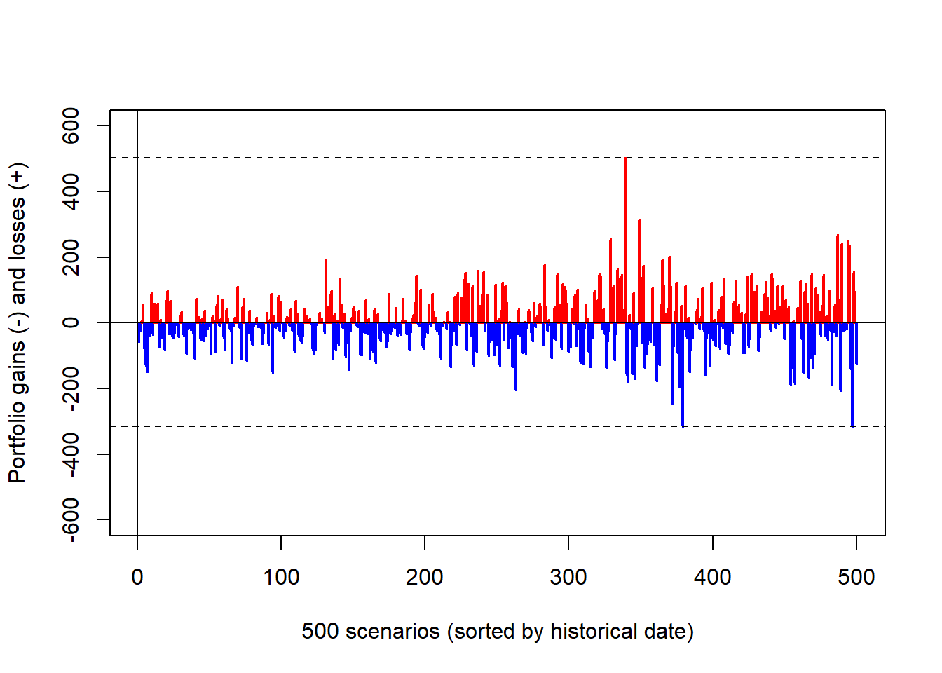
The scenario-loss plot preserves the historical ordering of the 500 daily changes. Positive bars are losses and negative bars are gains, so the picture gives a quick sense of the downside tail before selecting a VaR threshold.
Code
plot(l, type = "h", lwd = 2,
     xlab = "500 scenarios (sorted by historical date)",
     ylab = "Portfolio gains (-) and losses (+)",
     col = ifelse(l < 0, "blue", "red"))
points(501, l.tomorrow, pch = 19, cex = 2)
abline(0, 0)
abline(v = 0)
lines(seq(0, max(l, na.rm = TRUE), length.out = 500), lty = 2)
lines(seq(0, min(l, na.rm = TRUE), length.out = 500), lty = 2)
abline(h = 253.385, lwd = 2, col = "green")
legend("bottomleft", legend = c("Gains", "Losses", "Historical VaR: 253.385"),
       col = c("blue", "red", "green"), lty = 1, bg = "white", lwd = 2)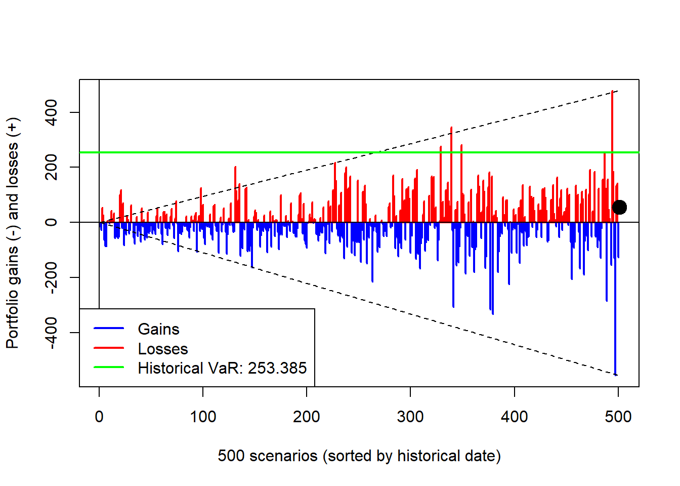
The histogram compresses the same scenarios into a distribution of losses. Most scenarios are clustered around moderate gains or losses, while VaR is read from the right tail.
Code
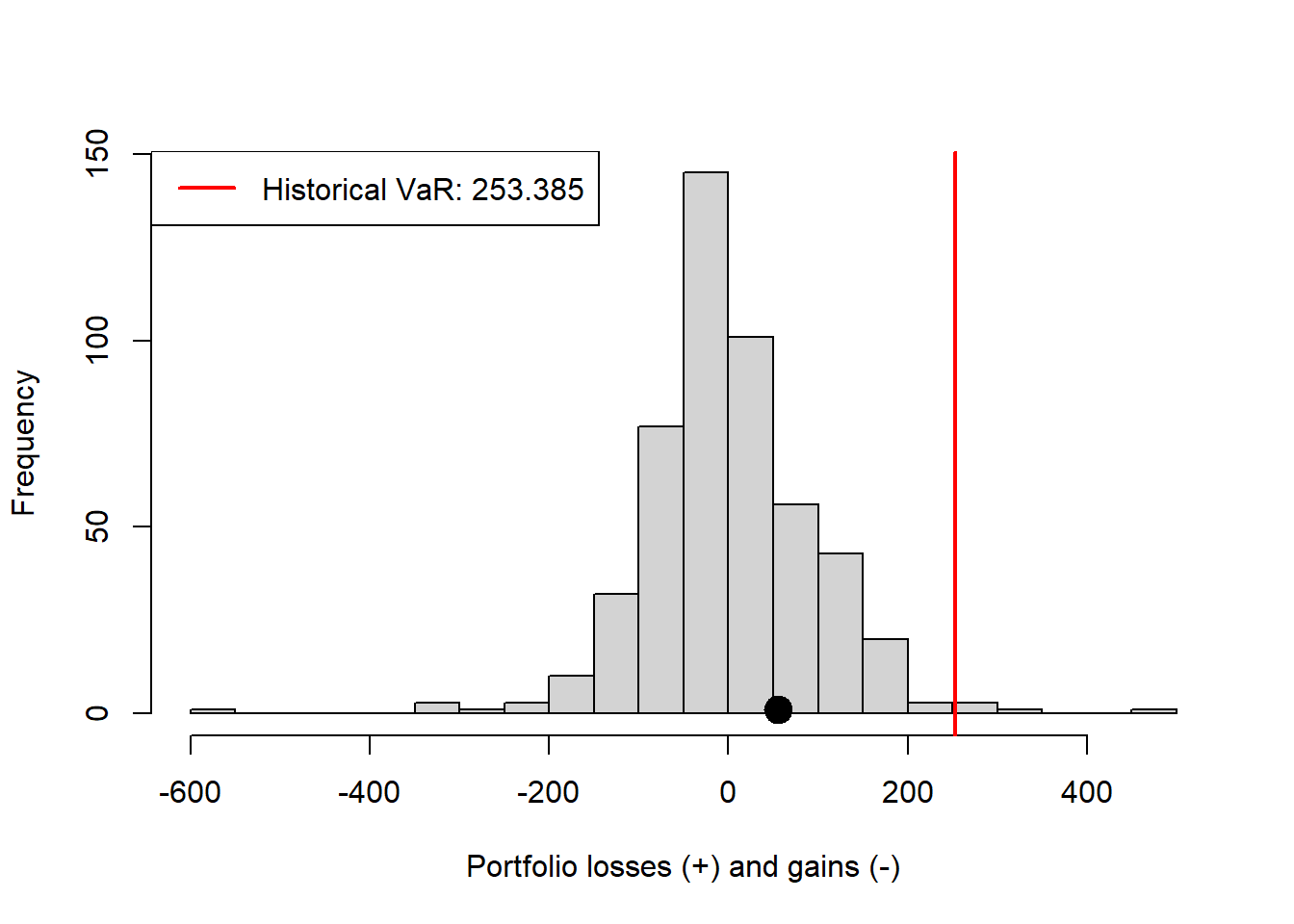
The point marks the realized loss, and the red line marks the historical VaR estimate. The density plot smooths the same information and makes the shape of the empirical loss distribution easier to compare with the normal model used later.
Code
densi <- density(l, na.rm = TRUE)
plot(densi, main = "", xlab = "Portfolio losses (+) and gains (-)")
polygon(densi, col = "grey", border = "black")
points(l.tomorrow, 0, pch = 19, cex = 2)
abline(v = 253.385, col = "red", lwd = 2)
legend("topleft", legend = c("Historical VaR: 253.385"), col = "red",
       bg = "white", lwd = 2)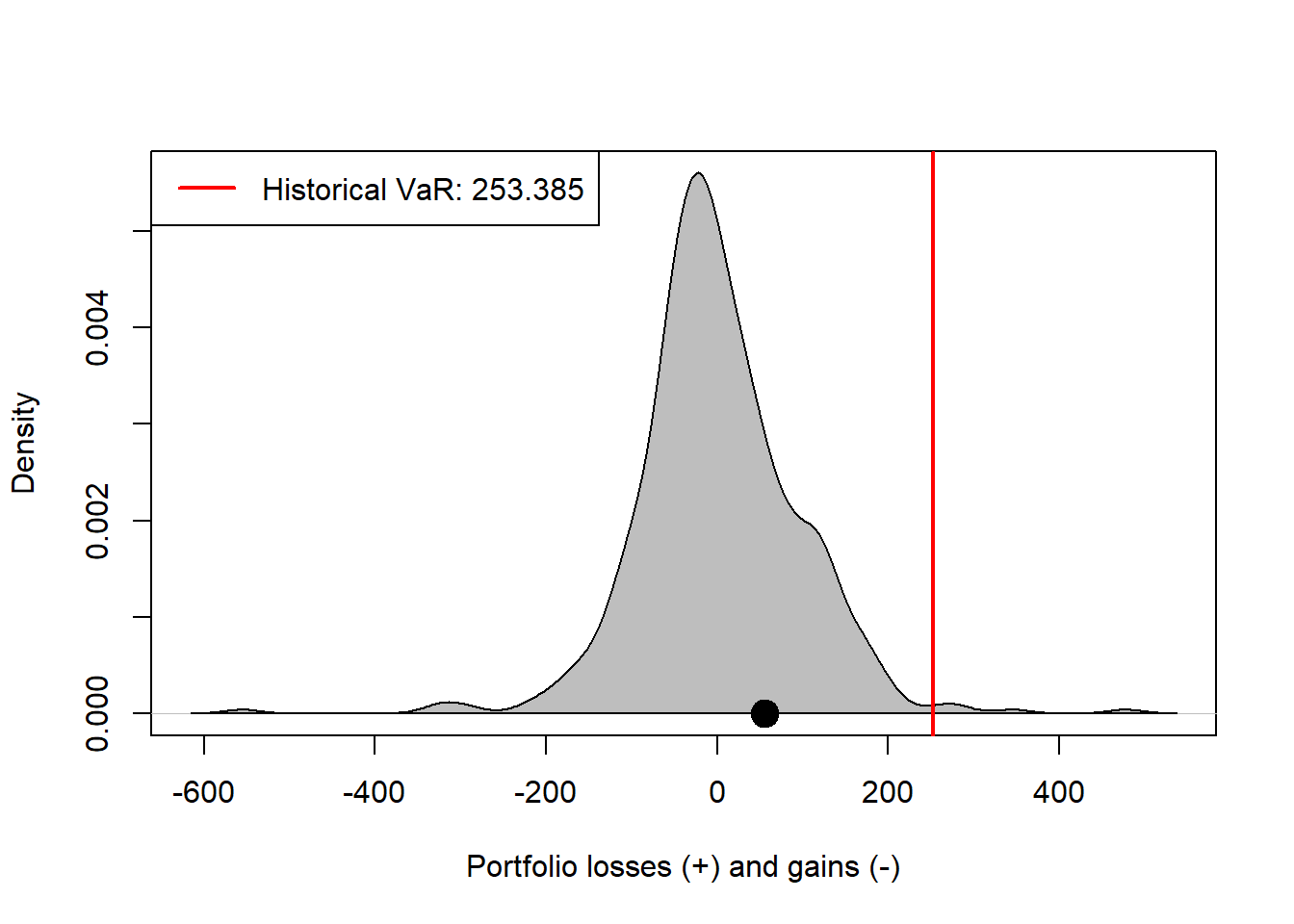
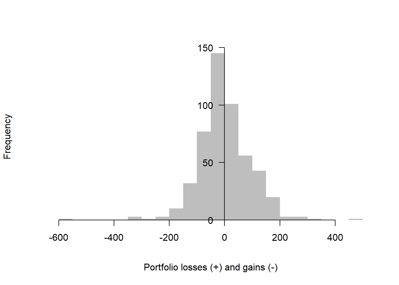
The same loss distribution can be displayed with axes that match the original textbook presentation.
Code
Ranking the 500 scenario losses from highest to lowest makes the tail selection explicit. At the 99% confidence level with 500 scenarios, 1% of the sample corresponds to five observations. The fifth-largest loss is therefore the discrete historical VaR used in the textbook example.
Code
     scenario.number loss.in.positive.values
l494             494                477.8410
l339             339                345.4351
l349             349                282.2038
l329             329                277.0413
l487             487                253.3850
l227             227                217.9740
l131             131                202.2555
l238             238                201.3892
l473             473                191.2691
l306             306                191.0497
l477             477                185.1269
l495             495                184.4496
l376             376                182.7072
l237             237                180.1048
l365             365                172.2237
The last values show the largest gains in the ranked loss table.
     scenario.number loss.in.positive.values
l395             395               -224.5146
l489             489               -284.9247
l341             341               -307.9301
l377             377               -316.4893
l379             379               -333.0218
l497             497               -555.7954
One of the highest gains happens in scenario 497, almost at the end of the historical window. The largest gains remain outside the VaR tail calculation and still help show that the historical window contains both downside and upside shocks.
Code
                               VaR.method     VaR
1 Historical simulation, original weights 253.385
The original weights are 40% in the DJIA, 30% in the FTSE, 10% in the CAC, and 20% in the Nikkei. They are treated as a benchmark allocation because they are assigned exogenously in the example. The ranked-loss barplot makes the 1% tail visible and separates the VaR estimate from the realized next-day outcome.
Code
barplot(l[order(l, decreasing = TRUE)],
        names.arg = order(l, decreasing = TRUE), ylim = c(0, 500),
        xlim = c(0, 20), las = 2, cex.names = 1, ylab = "Portfolio loss ($000s)",
        col = "red", xlab = "Scenario number (ranked)")
abline(h = 253.385, lwd = 3)
abline(h = 0, lwd = 3)
abline(h = l.tomorrow, lwd = 3, col = "green")
legend("topright", legend = c("Historical VaR: 253.385",
       "Realized loss"), col = c("black", "green"),
       bg = "white", lwd = 2)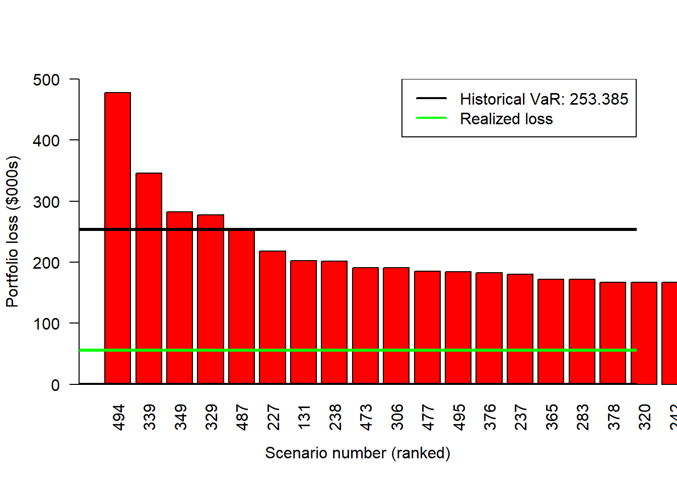
The top 1% can also be explored with the quantile() function. R’s default quantile estimator interpolates between order statistics, so its 99% value differs from Hull’s fifth-worst-scenario historical VaR. The difference comes from a numerical convention for estimating sample quantiles.
Hull’s discrete historical VaR is reproduced by taking the fifth largest loss directly.
The default quantile() function at the 99% level gives the interpolated estimate.
The quantile curve shows how the VaR estimate changes with the confidence level.
Code
plot(seq(from = 0.902, to = 1, by = 0.002),
     quantile(l, seq(from = 0.902, to = 1, by = 0.002)), cex = 1.5,
     xlab = "Confidence level (vertical line at 99%)",
     ylab = "Portfolio VaR")
abline(v = 0.99, lty = 2, lwd = 2)
abline(h = quantile(l, 0.99), col = "blue", lty = 2, lwd = 2)
abline(h = Table22.4[5, 2], col = "red", lty = 2, lwd = 2)
legend("topleft", legend = c("99% level", "Historical VaR: 253.385",
                             "99% quantile VaR: 218.3281"),
       col = c("black", "red", "blue"), lty = 2, bg = "white", lwd = 2)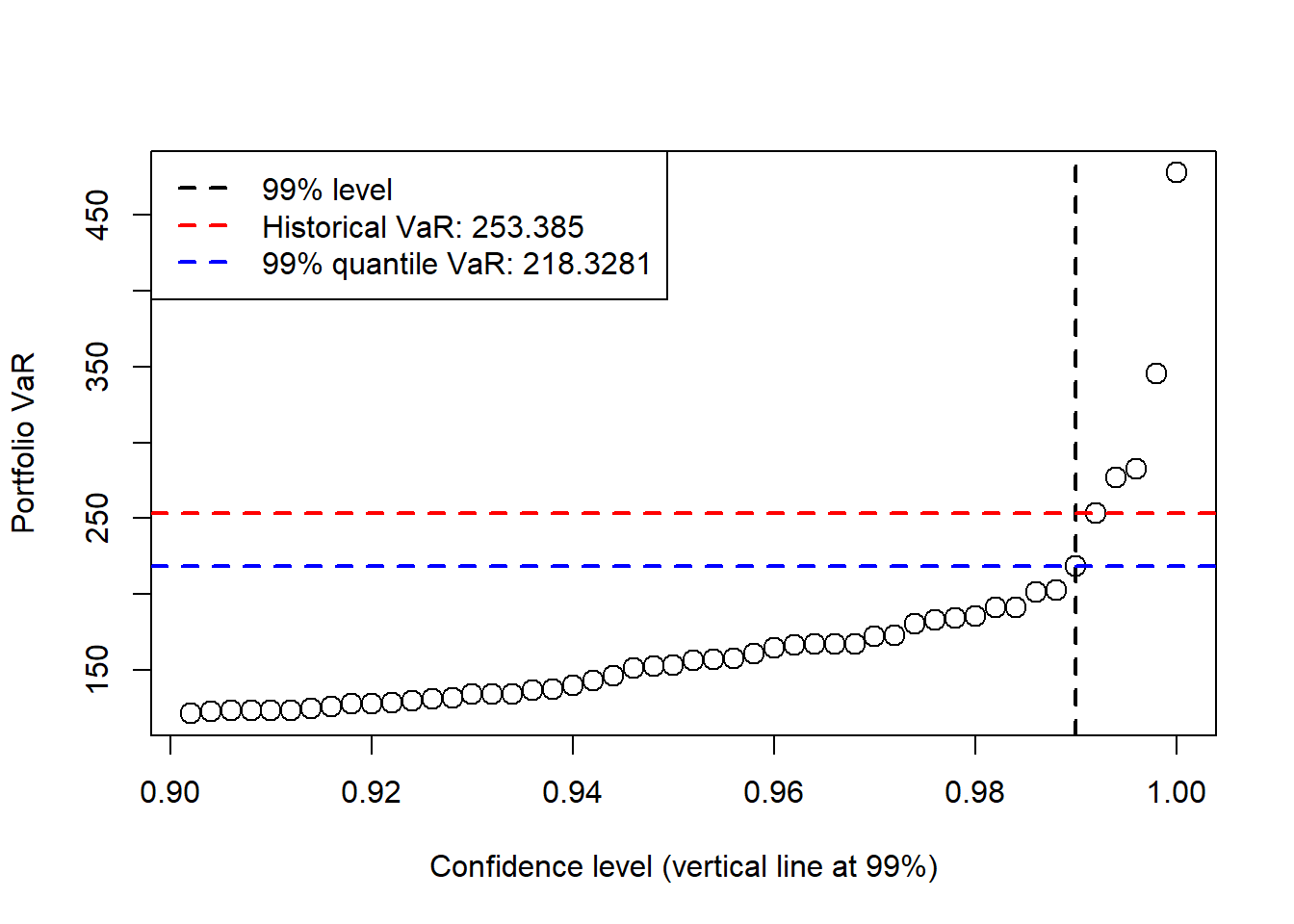
Code
             quantile.function scenario.number sort.losses
98.9979960%           217.9740             227    217.9740
99.1983968%           253.3850             487    253.3850
99.3987976%           277.0413             329    277.0413
99.5991984%           282.2038             349    282.2038
99.7995992%           345.4351             339    345.4351
100.0000000%          477.8410             494    477.8410
The results table stores the historical VaR estimates.
Code
                                           VaR.method      VaR
1 Historical approximate quantile(), original weights 218.3281
2             Historical simulation, original weights 253.3850
6.3 Model building approach
The model-building approach assumes normality for portfolio losses. The historical loss distribution can deviate from that assumption, especially in the tails. Its main advantage is simplicity: once the covariance matrix and portfolio weights are defined, VaR follows from the normal quantile. The method is also useful as a benchmark against historical simulation because both methods use the same portfolio and horizon.
The adjusted indices are first transformed into simple returns.
\[ R_{j,t}=\frac{S_{j,t}-S_{j,t-1}}{S_{j,t-1}}. \]
Code
R <- df.Adj %>%
  select(Day, DJIA, AFTSE100, ACAC40, ANikkei) %>%
  mutate(RDJIA = (DJIA-lag(DJIA))/lag(DJIA)) %>%
  mutate(RFTSE100 = (AFTSE100-lag(AFTSE100))/lag(AFTSE100)) %>%
  mutate(RCAC40 = (ACAC40-lag(ACAC40))/lag(ACAC40)) %>%
  mutate(Nikkei = (ANikkei-lag(ANikkei))/lag(ANikkei)) %>%
  select(RDJIA, RFTSE100, RCAC40, Nikkei) %>%
  slice(-1)

R.tomorrow <- R %>%
  slice(501)

R <- R %>%
  slice(-501)
The correlation matrix on September 25, 2008 is calculated by giving equal weight to the last 500 daily returns.
               RDJIA  RFTSE100    RCAC40      Nikkei
RDJIA     1.00000000 0.4891059 0.4957096 -0.06189921
RFTSE100  0.48910594 1.0000000 0.9181083  0.20094221
RCAC40    0.49570963 0.9181083 1.0000000  0.21095096
Nikkei   -0.06189921 0.2009422 0.2109510  1.00000000
The covariance matrix on September 25, 2008 is calculated by giving equal weight to the last 500 daily returns.
                 RDJIA     RFTSE100       RCAC40        Nikkei
RDJIA     1.229524e-04 7.696591e-05 7.682514e-05 -9.493488e-06
RFTSE100  7.696591e-05 2.013973e-04 1.821076e-04  3.944302e-05
RCAC40    7.682514e-05 1.821076e-04 1.953506e-04  4.078130e-05
Nikkei   -9.493488e-06 3.944302e-05 4.078130e-05  1.913129e-04
This covariance matrix is close to the one in Hull (2015). Minor differences arise because the calculations here do not use rounded intermediate values.
With dollar allocations \(\alpha=(4000,3000,1000,2000)'\), the variance of portfolio losses in thousands of dollars follows the quadratic portfolio-risk expression.
\[ \sigma_p^2=\alpha'\Sigma\alpha. \]
Code
         [,1]
[1,] 8779.392
Hull reports 8,761.833 for this variance. The value calculated here is slightly different because the code keeps more intermediate precision. Taking the square root gives the portfolio standard deviation.
The one-day 99% VaR under the normal model multiplies the portfolio standard deviation by the 99% normal quantile.
\[ VaR_{0.99}=z_{0.99}\sigma_p. \]
Hull reports $217,757. In the units used here, that is 217.757 in thousands of dollars, compared with 253.385 from the historical simulation approach. The model-building estimate is lower in this case because the normal approximation smooths the empirical tail.
Code
                                                  VaR.method      VaR
1        Historical approximate quantile(), original weights 218.3281
2                    Historical simulation, original weights 253.3850
3 Model building equal observation weights, original weights 217.9751
The equal-observation-weight covariance estimate can be compared with the exponentially weighted moving average method (EWMA).
With decay parameter \(\lambda\) and demeaned return vector \(u_t=r_t-\bar r\), the EWMA covariance update gives more weight to recent squared return innovations.
\[ \Sigma_t=\lambda\Sigma_{t-1}+(1-\lambda)u_{t-1}u_{t-1}'. \]
Code
# Model building example -- EWMA
covEWMA <-
  function(factors, lambda = 0.96, return.cor = FALSE) {
    factor.names  = colnames(factors)
    t.factor      = nrow(factors)
    k.factor      = ncol(factors)
    factors       = as.matrix(factors)
    t.names       = rownames(factors)
    factor.means  = colMeans(factors)

    cov.f.ewma = array(,c(t.factor, k.factor, k.factor))
    cov.f = var(factors)  # unconditional variance as EWMA at time = 0
    FF = (factors[1, ] - factor.means) %*% t(factors[1,] - factor.means)
    cov.f.ewma[1,,] = (1 - lambda) * FF  + lambda * cov.f
    for (i in 2:t.factor) {
    FF = (factors[i, ] - factor.means) %*% t(factors[i, ] - factor.means)
    cov.f.ewma[i,,] = (1 - lambda) * FF  + lambda * cov.f.ewma[(i-1),,]
    }
    dimnames(cov.f.ewma) = list(t.names, factor.names, factor.names)

    if(return.cor) {
      cor.f.ewma = cov.f.ewma
      for (i in 1:dim(cor.f.ewma)[1]) {
        cor.f.ewma[i, , ] = cov2cor(cov.f.ewma[i, ,])
      }
      return(cor.f.ewma)
    } else {
      return(cov.f.ewma)
    }
  }
The covariance matrix on September 25, 2008 is also calculated using the EWMA method with \(\lambda=0.94\). EWMA gives more weight to recent observations, so it responds more strongly when volatility rises near the end of the sample.
                 RDJIA     RFTSE100       RCAC40        Nikkei
RDJIA     0.0004801472 0.0004300030 0.0004257243 -0.0000398876
RFTSE100  0.0004300030 0.0010311334 0.0009630006  0.0002090981
RCAC40    0.0004257243 0.0009630006 0.0009535706  0.0001681154
Nikkei   -0.0000398876 0.0002090981 0.0001681154  0.0002534478
The variance of portfolio losses again follows the quadratic form \(\alpha'\Sigma\alpha\).
Hull reports 40,995.765 for this value. Taking the square root gives the EWMA portfolio standard deviation.
Hull reports 202.474 for this value. The one-day 99% VaR is therefore calculated from the same normal-quantile expression used above.
Hull reports $471,025, or 471.025 in thousands of dollars. This value is more than twice the VaR estimated with equal observation weights, which reflects the higher volatility near the end of the sample.
Code
                                                  VaR.method      VaR
1        Historical approximate quantile(), original weights 218.3281
2                    Historical simulation, original weights 253.3850
3                      Model building EWMA, original weights 470.9187
4 Model building equal observation weights, original weights 217.9751
The table compares daily volatilities under equal observation weights and EWMA.
Code
                       DJIA FTSE 100   CAC 40 Nikkei 225
Equal obs. weights 1.108839 1.419145 1.397679   1.383159
EWMA               2.191226 3.211127 3.087994   1.592004
The estimated daily standard deviations are much higher when EWMA is used than when data receive equal observation weights. This happens because volatilities were much higher during the period immediately preceding September 25, 2008, than during the rest of the 500 days covered by the data.
6.4 Optimal allocation
VaR depends on the loss distribution, and the loss distribution depends on the weights. The current benchmark portfolio weights provide the reference allocation.
Code
            DJIA FTSE 100 CAC 40 Nikkei 225
W_benchmark  0.4      0.3    0.1        0.2
The following calculation estimates three comparison portfolios: the benchmark allocation, a minimum-variance allocation, and an allocation that targets the expected return of the CAC 40. Returns are expressed in percent for the mean-variance exercise; the later VaR calculations continue to use dollar allocations and the unscaled covariance matrices.
The minimum-variance allocation solves a constrained variance minimization problem.
\[ \min_w w'\Sigma w \quad \text{subject to} \quad \mathbf{1}'w=1. \]
The CAC 40 target-return allocation adds a return constraint to the same variance minimization problem. This analytical Markowitz calculation is unconstrained, so a target-return solution can include negative weights. In portfolio language, a negative weight is a short position.
\[ \min_w w'\Sigma w \quad \text{subject to} \quad \mathbf{1}'w=1,\quad w'\mu=\mu_{CAC40}. \]
Code
R <- R * 100
R.tomorrow <- R.tomorrow * 100
stocks<- c("DJIA", "FTSE100", "CAC40", "Nikkei")
sigma <- var(R)
sd <- diag(sigma)^0.5
E <- colMeans(R)
E.tomorrow <- colMeans(R.tomorrow)
ones <- abs(E / E)
a <- c(t(ones) %*% solve(sigma) %*% ones)
b <- c(t(ones) %*% solve(sigma) %*% E)
c <- c(t(E) %*% solve(sigma) %*% E)
d <- c(a * c - (b^2))
g <- c(solve(sigma) %*% (c * ones - b * E) / d)
h <- c(solve(sigma) %*% (a * E - b * ones) / d)
ER <- seq(from = -0.3, to = 0.3, by = 0.0001)
S <- ER
W <- matrix(0, nrow = length(ER), ncol = length(stocks))
for(i in 1:length(ER)){
  W[i,] <- g + h * ER[i]
  ER[i] <- W[i,] %*% E
  S[i] <- (t(W[i,]) %*% sigma %*% W[i, ])^0.5
  }
W_min <- (solve(sigma) %*% ones) / a
R_min <- c(t(W_min) %*% E)
R_min.realized <- c(t(W_min) %*% E.tomorrow)
S_min <- c(t(W_min) %*% sigma %*% W_min)^0.5
# Allocation targeting the CAC40 expected return with lower estimated variance.
W.cac40 <- g + h * E[3]
R_cac40 <- c(t(W.cac40) %*% E)
R_cac40.realized <- c(t(W.cac40) %*% E.tomorrow)
S_cac40 <- c(t(W.cac40) %*% sigma %*% W.cac40)^0.5
R_benchmark.realized = c(t(W_benchmark) %*% E.tomorrow)
There are now four portfolio-weight alternatives, two of which are optimized. The risk-management comparison asks whether optimized weights reduce VaR under the same data and horizon.
Code
                         DJIA    FTSE 100     CAC 40 Nikkei 225
Benchmark weights   0.4000000  0.30000000 0.10000000  0.2000000
minimum variance    0.5592378  0.03793305 0.02279301  0.3800361
CAC40 target return 0.6075003 -0.40341894 0.45978629  0.3361323
equal 1/N           0.2500000  0.25000000 0.25000000  0.2500000
The portfolio weights remain constant in this worked example. A dynamic implementation could rebalance weights as new data arrive. The following resource shows the time evolution of minimum-variance weights when five US industry portfolios are used as investment assets.
A similar exercise with 10 US industry-sorted portfolios extends the same idea.
The comparison now returns to the four-index portfolio.
Code
W_benchmark <- alpha / 10000
R_benchmark <- c(t(W_benchmark) %*% E)
S_benchmark <- c(t(W_benchmark) %*% sigma %*% W_benchmark)^0.5

plot(S, ER, type = "l", lwd = 3, xlim = c(0.7, 1.6),
     ylim = c(-0.022, 0.005),
     ylab = "Expected return", xlab = "Standard deviation")
points(diag(sigma)^0.5, E)
abline(0, R_benchmark / S_benchmark, lty = 3, col = "blue")
abline(0, R_min / S_min, lty = 3, col = "red")
points(S_min, R_min, col = "red", pch = 19, cex = 2)
abline(0, 0, lty = 3)
text(S_min, R_min, "Minimum
     variance", pos = 2, cex = 0.8)
text(sd, E, stocks, adj = -0.5, cex = 0.8)
points(S_benchmark, R_benchmark, col = "blue", pch = 19, cex = 2)
text(S_benchmark, R_benchmark, "Benchmark
     allocation", adj = -0.3, cex = 0.8, pos = 1)
legend("bottomleft",
       legend = c("DJ=0.4,   FTSE=0.3,     CAC=0.1,     Nikkei=0.2",
                            "DJ=0.56, FTSE=0.038, CAC=0.022, Nikkei=0.38"),
       col = c("blue", "red"), pch = 19, bg = "white", cex = 1)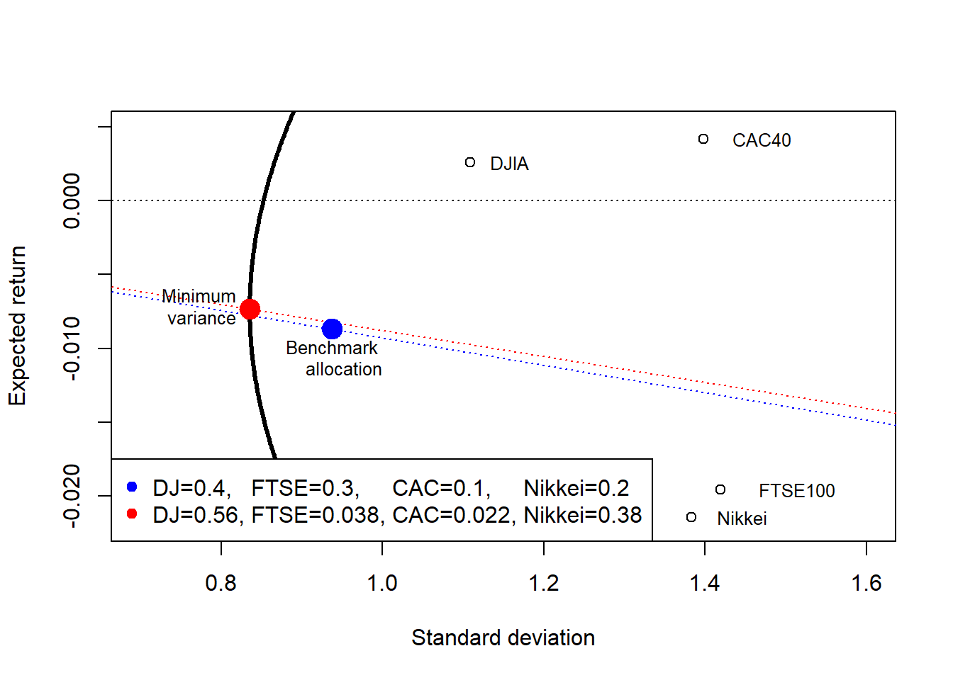
The figure suggests that the minimum-variance alternative reduces estimated portfolio risk relative to the original allocation. In the estimated mean-variance space, the minimum-variance portfolio has higher expected return and lower estimated risk. The statement is in-sample and based on estimated means and covariances. The realized outcome can then be evaluated with the actual returns for September 26, 2008.
[1] 0.2629549[1] -0.5583249The comparison suggests that the original allocation would have produced a realized return of -0.5583249% on Friday September 26, 2008. The minimum-variance allocation would have produced a portfolio gain of 0.2629549%. The example shows why portfolio weights matter before VaR is computed: the loss distribution changes when the allocation changes.
Code
W_benchmark <- alpha / 10000
R_benchmark <- c(t(W_benchmark) %*% E)
S_benchmark <- c(t(W_benchmark) %*% sigma %*% W_benchmark)^0.5

W_1N <- c(0.25,0.25,0.25,0.25)
R_1N <- c(t(W_1N) %*% E)
S_1N <- c(t(W_1N) %*% sigma %*% W_1N)^0.5

plot(S, ER, type = "l", lwd = 3, xlim = c(0.7, 1.6),
     ylim = c(-0.022, 0.005),
     ylab = "Expected return", xlab = "Standard deviation")
points(diag(sigma)^0.5, E)
abline(0, R_benchmark / S_benchmark, lty = 3, col = "blue")
abline(0, R_min / S_min, lty = 3, col = "red")
abline(0, R_1N / S_1N, lty = 3, col = "purple")
points(S_min, R_min, col = "red", pch = 19, cex = 2)
points(S_1N, R_1N, col = "purple", pch = 19, cex = 2)
abline(0, 0, lty = 3)
text(S_min, R_min, "Minimum
     variance", pos = 2, cex = 0.8)
text(sd, E, stocks, adj = -0.5, cex = 0.8)
points(S_benchmark, R_benchmark, col = "blue", pch = 19, cex = 2)
text(S_benchmark, R_benchmark, "Benchmark
     allocation", adj = -0.3, cex = 0.8, pos = 1)
text(S_1N, R_1N, "1/N", adj = -0.3, cex = 0.8, pos = 3)
legend("bottomleft",
       legend =
         c("Bench.: DJ=0.4,   FTSE=0.3,     CAC=0.1,     Nikkei=0.2",
"Minvar: DJ=0.56, FTSE=0.038, CAC=0.022, Nikkei=0.38",
"1/N:      DJ=0.25,  FTSE=0.25,  CAC=0.25,  Nikkei=0.25"),
       col = c("blue","red", "purple"), pch = 19,
bg = "white", cex = 0.9)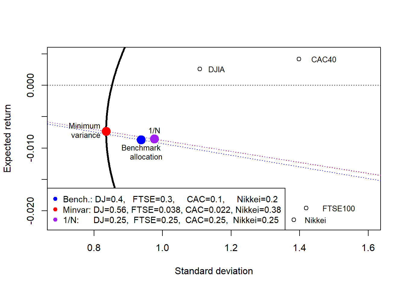
The efficient frontier also changes when the investable universe changes. The following resource shows the US efficient frontier using five industry-sorted portfolios as investment assets.
Increasing the number of investment assets can expand the mean-variance frontier when the added assets bring useful return, risk, or correlation characteristics. The following resource compares 10 versus 12 US industry-sorted portfolios.
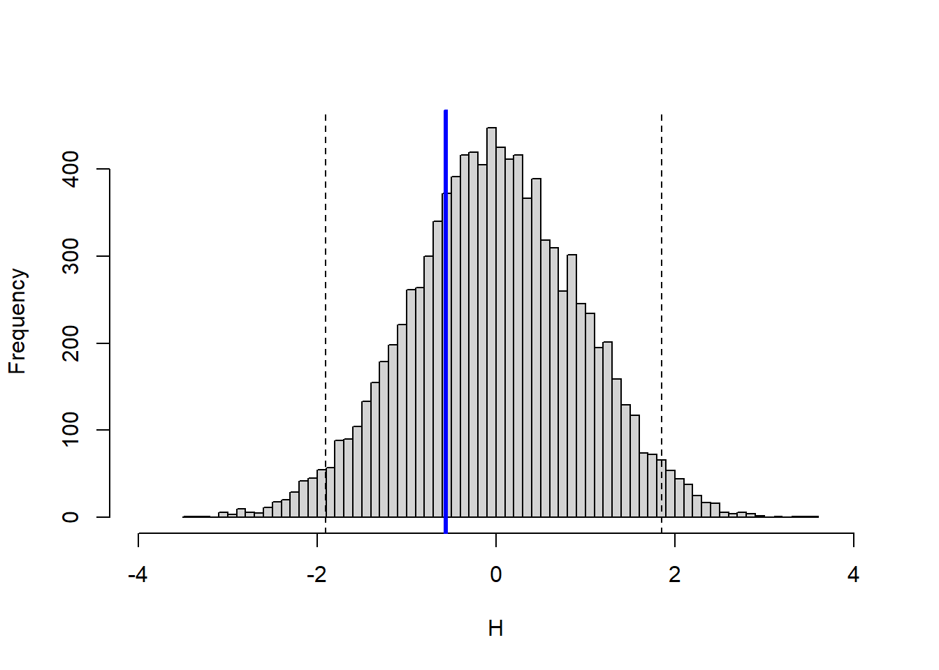
The mean and standard deviation estimates can also be used to simulate 10,000 possible one-day returns for Friday September 26, 2008. The histograms below are model-based checks of where the realized return falls relative to the fitted normal distribution.
The first simulated distribution corresponds to the minimum-variance portfolio.
Code
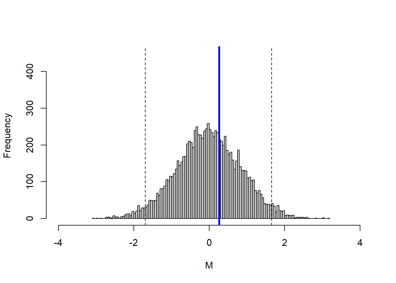
The blue line falls on the gain side of the simulated distribution. For this particular day, the minimum-variance allocation produced a positive realized return under the observed market moves.
The second simulated distribution corresponds to the original allocation.
Code
The blue line for the original allocation falls on the loss side. Comparing this histogram with the previous one shows that changing the weights changes both the center of the fitted distribution and the realized portfolio return.
The portfolio that targets the CAC 40 expected return is evaluated in the same way.
Code

The CAC 40 target-return allocation also produces a positive realized return in this one-day evaluation. Because this allocation uses a negative FTSE weight, its apparent improvement has to be read together with short-selling feasibility and implementation constraints.
The portfolio that targets the CAC 40 expected return can also be located in mean-variance space.
Code
plot(S, ER, type = "l", lwd = 3, xlim = c(0.7, 1.6),
     ylim = c(-0.022, 0.007), ylab = "Expected return",
     xlab = "Standard deviation")
points(diag(sigma)^0.5, E)
abline(0, 0, lty = 3)
points(S_cac40, R_cac40, col = "red", pch = 19, cex = 2)
points(0.68, R_cac40.realized, col = "red", pch = 15, cex = 2)
text(S_cac40, R_cac40, "CAC40
     expected return", pos = 2, cex = 0.8)
text(sd,E,stocks,adj=-0.5,cex=0.8)
W_benchmark = alpha / 10000
R_benchmark = c(t(W_benchmark) %*% E)
S_benchmark = c(t(W_benchmark) %*% sigma %*% W_benchmark)^0.5
points(S_benchmark, R_benchmark, col = "blue", pch = 19, cex = 2)
points(0.68, R_benchmark.realized, col = "blue", pch = 15, cex = 2)
abline(0,R_benchmark / S_benchmark, lty = 3, col = "blue")
abline(0,R_cac40 / S_cac40, lty = 3, col = "red")
abline(0,E[3] / sd[3], lty = 3)
abline(v = S_cac40, lty = 3)
text(S_benchmark, R_benchmark, "Benchmark
     allocation", adj = -0.3, cex = 0.8, pos = 1)
legend("bottomleft",
       legend = c("DJ=0.4,     FTSE=0.3,      CAC=0.1,     Nikkei=0.2",
                          "DJ=0.607, FTSE=-0.403, CAC=0.459, Nikkei=0.336"), col = c("blue", "red"),
       pch = 19, bg = "white", cex = 0.9)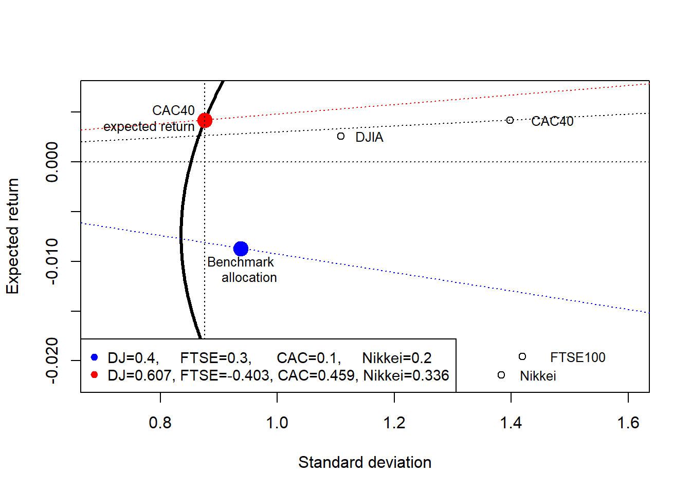
The realized returns on Friday September 26, 2008 are used to compare the three allocations.
[1] 0.2629549[1] -0.5583249[1] 0.5183212The original portfolio allocation produces a loss on the realized day. It would lead to a return of -0.558%, equivalent to a loss of 0.558%. The minimum-variance allocation would lead to a positive return of 0.2629%, and the portfolio that targets the CAC 40 expected return leads to a realized return of 0.518%. The last case uses a short FTSE position, so it requires additional feasibility checks before being interpreted as an implementable allocation.
6.5 Model building approach with optimal weights
The two optimized portfolios are evaluated with the model-building VaR approach. This keeps the covariance estimate fixed and changes only the portfolio weights, which isolates the effect of allocation on VaR. For any weight vector \(w\), the dollar allocation is \(\alpha(w)=10{,}000w\) in thousands of dollars and the normal VaR is
\[ VaR_{0.99}(w)=z_{0.99}\sqrt{\alpha(w)'\Sigma\alpha(w)}. \]
Code
# Model-building approach with equal observation weights.
alpha2 <- c(W_min * 10000)
alpha3 <- c(W.cac40 * 10000)
# Minimum-variance optimal portfolio.
Pvar2 <- t(alpha2) %*% Rcov %*% alpha2
Psd2 <- Pvar2^0.5
VaR.ew.optimal <- qnorm(0.99, 0, 1) * Psd2
# CAC 40 target-return optimal portfolio.
Pvar3 <- t(alpha3) %*% Rcov %*% alpha3
Psd3 <- Pvar3^0.5
VaR.ew.optimal.cac <- qnorm(0.99, 0, 1) * Psd3
The results table includes the model-building VaR estimates with optimal weights.
Code
                                                          VaR.method      VaR
1                Historical approximate quantile(), original weights 218.3281
2                            Historical simulation, original weights 253.3850
3                              Model building EWMA, original weights 470.9187
4 Model building equal observation weights, minimum variance weights 194.3892
5         Model building equal observation weights, original weights 217.9751
6          Model building equal observation weights, targeting CAC40 203.7821
The second calculation uses the EWMA covariance matrix.
Code
         [,1]
[1,] 338.3195
Code
         [,1]
[1,] 348.1888
The results table includes the EWMA VaR estimates with optimal weights.
Code
                                                          VaR.method      VaR
1                Historical approximate quantile(), original weights 218.3281
2                            Historical simulation, original weights 253.3850
3                      Model building EWMA, minimum variance weights 338.3195
4                              Model building EWMA, original weights 470.9187
5                               Model building EWMA, targeting CAC40 348.1888
6 Model building equal observation weights, minimum variance weights 194.3892
7         Model building equal observation weights, original weights 217.9751
8          Model building equal observation weights, targeting CAC40 203.7821
6.6 Historical approach with optimal weights
The final comparison returns to historical simulation and applies the same scenario returns to the optimized weights. This keeps the market scenarios fixed and changes only the portfolio exposure. For 500 scenarios, the empirical 99% VaR is again the fifth-worst loss.
\[ VaR_{0.99}^{hist}(w)=l_{(5)}(w), \]
where losses are sorted from largest to smallest.
Code
df.Adj.S <- df.Adj.S %>%
  mutate(p2 = (alpha2[1] * SDJIA / DJIA[501]) +
             (alpha2[2] * SFTSE100 / AFTSE100[501]) +
             (alpha2[3] * SCAC40 / ACAC40[501]) +
             (alpha2[4] * SNikkei / ANikkei[501])) %>%
  mutate(l2 = 10000 - p2) %>% # Losses l
  mutate(p3 = (alpha3[1] * SDJIA / DJIA[501]) +
             (alpha3[2] * SFTSE100 / AFTSE100[501]) +
             (alpha3[3] * SCAC40 / ACAC40[501]) +
             (alpha3[4] * SNikkei / ANikkei[501])) %>%
  mutate(l3 = 10000 - p3) # Losses l
The new portfolio losses are calculated under the optimized weights.
Code
The benchmark allocation provides the reference distribution.
Code
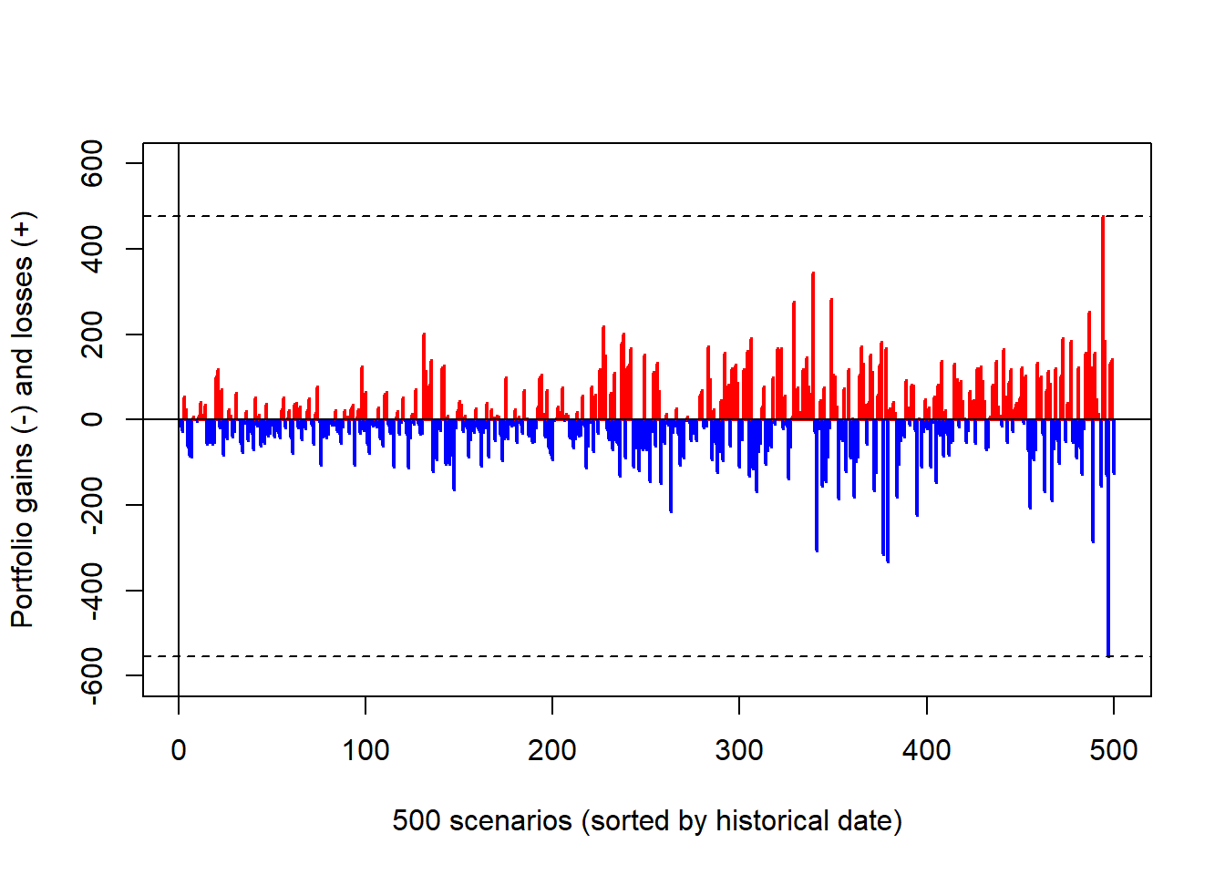
The benchmark distribution contains several large downside scenarios, and the fifth-worst loss is the historical 99% VaR for the original allocation.
The one-day 99% value at risk can be estimated as the fifth-worst loss.
The historical approach is then applied with minimum-variance weights.
Code
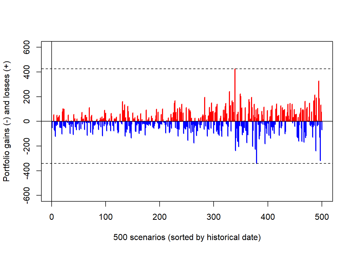
The range of losses and gains is reduced under the minimum-variance weights. The one-day 99% Value at Risk can be estimated as the fifth-worst loss.
The results table is updated with this case.
Code
                                                          VaR.method      VaR
1                Historical approximate quantile(), original weights 218.3281
2                    Historical simulation, minimum variance weights 213.6898
3                            Historical simulation, original weights 253.3850
4                      Model building EWMA, minimum variance weights 338.3195
5                              Model building EWMA, original weights 470.9187
6                               Model building EWMA, targeting CAC40 348.1888
7 Model building equal observation weights, minimum variance weights 194.3892
8         Model building equal observation weights, original weights 217.9751
9          Model building equal observation weights, targeting CAC40 203.7821
The final case is the portfolio targeting the CAC 40 expected return.
Code
The CAC 40 target-return allocation also compresses much of the loss range while still allowing larger gains in some scenarios. The one-day 99% Value at Risk can be estimated as the fifth-worst loss. Because this portfolio includes a short FTSE position, its risk reduction is linked to an exposure that may be constrained in practice.
The results table is updated again.
Code
                                                           VaR.method      VaR
1                 Historical approximate quantile(), original weights 218.3281
2                     Historical simulation, minimum variance weights 213.6898
3                             Historical simulation, original weights 253.3850
4                              Historical simulation, targeting CAC40 248.8909
5                       Model building EWMA, minimum variance weights 338.3195
6                               Model building EWMA, original weights 470.9187
7                                Model building EWMA, targeting CAC40 348.1888
8  Model building equal observation weights, minimum variance weights 194.3892
9          Model building equal observation weights, original weights 217.9751
10          Model building equal observation weights, targeting CAC40 203.7821
The three historical approaches are compared side by side.
Code
par(mfrow=c(1, 3), oma = c(0, 0, 2, 0))
par(pty = "s")
plot(l, type = "h", ylim = c(-600, 600), lwd = 2, xlab = "",
     main = "Benchmark allocation",
     ylab = "Portfolio gains (-) and losses (+)",
     col = ifelse(l < 0, "blue", "red"))
abline(0, 0)
abline(v = 0)
abline(h = max(l), lty = 2)
abline(h = min(l), lty = 2)
plot(l2, type = "h", ylim = c(-600, 600), lwd = 2,
     main = "Minimum variance",
     xlab = "500 scenarios sorted by historical date", ylab = "",
     col = ifelse(l2 < 0, "blue", "red"))
abline(0, 0)
abline(v = 0)
abline(h = max(l2), lty = 2)
abline(h = min(l2), lty = 2)
plot(l3, type = "h", ylim = c(-600, 600), lwd = 2, xlab = "",
     main = "CAC40 target return", ylab = "",
     col = ifelse(l3 < 0, "blue", "red"))
abline(0, 0)
abline(v = 0)
abline(h = max(l3), lty = 2)
abline(h = min(l3), lty = 2)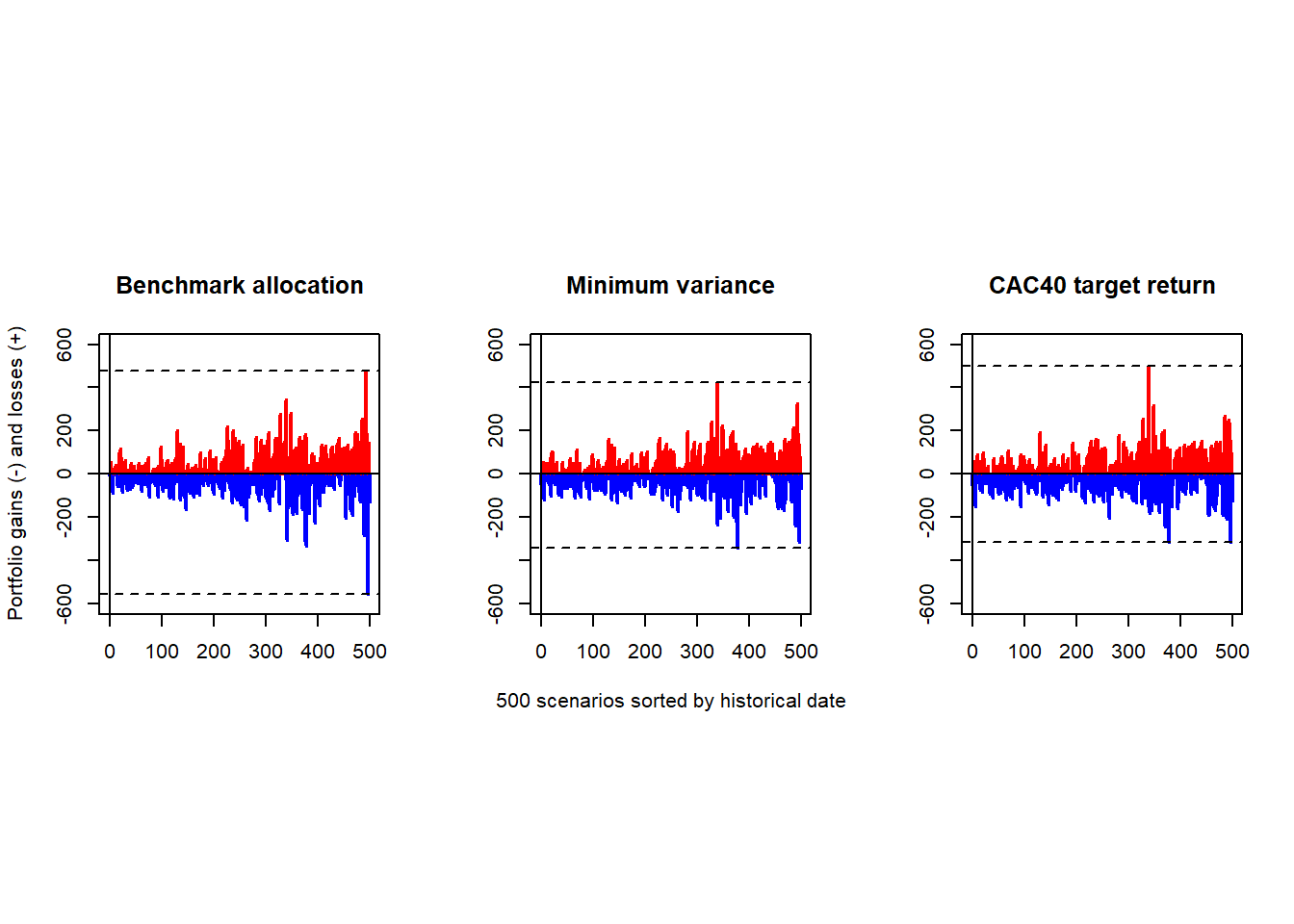
The side-by-side view makes the effect of allocation visible. The optimized portfolios reduce the height of the worst loss bars in this historical window, while the CAC 40 target-return case changes the distribution partly through the short FTSE exposure.
The quantiles provide a compact comparison of the three loss distributions.
Code
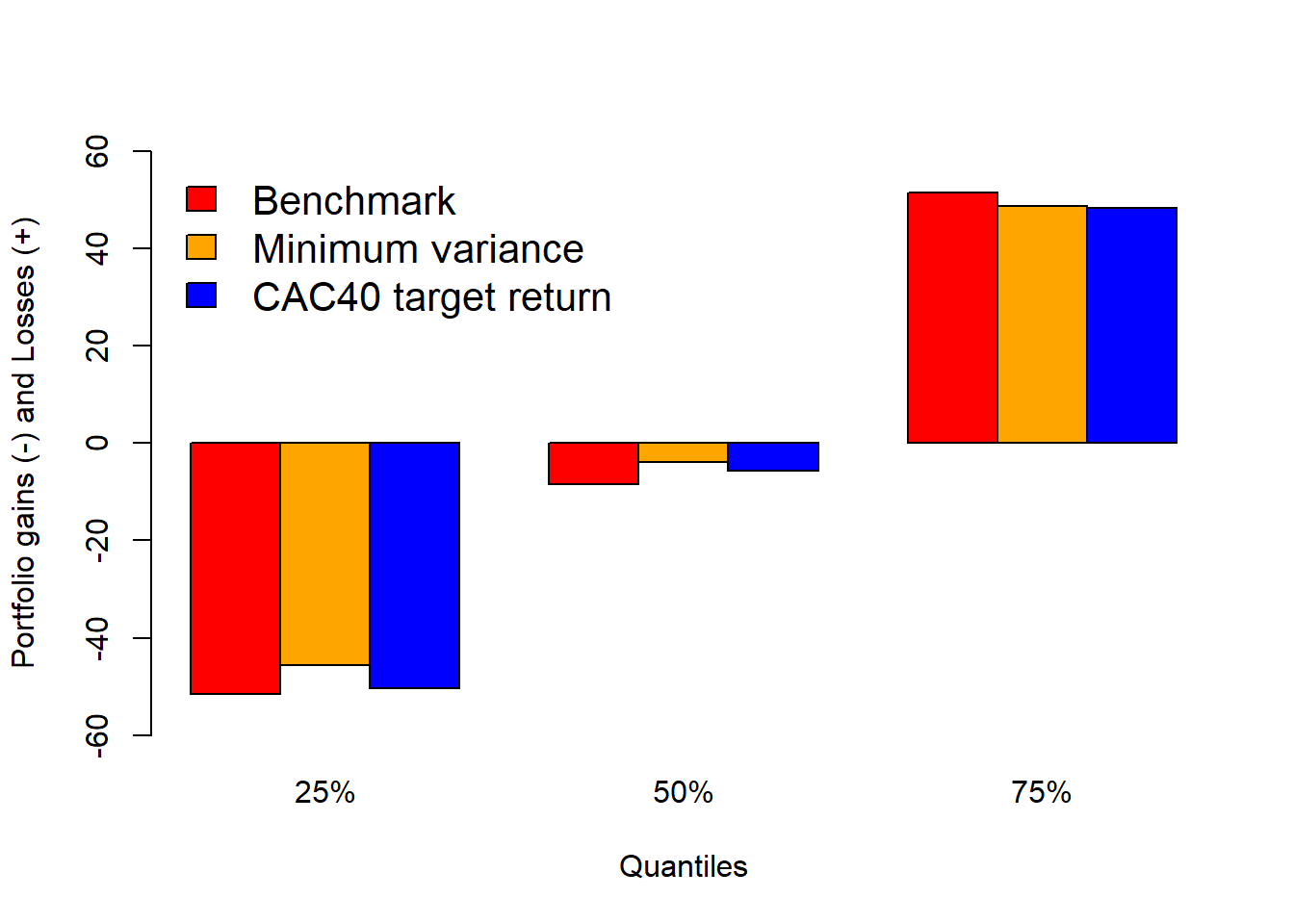
The quantile comparison summarizes the same message without the full time ordering of scenarios: changing weights shifts the empirical loss distribution, and VaR changes because it is a tail quantile of that distribution.
The chapter’s main value is integration. The VaR number is the final summary, after the analyst prepares international index data, converts foreign values into US dollars, defines portfolio weights, generates loss scenarios, estimates volatility and covariance inputs, compares allocation choices, and reads the realized outcome. Within the Financial Modeling with R path, VaR turns data, returns, allocation, and market-risk assumptions into a single loss statement that can be audited and recomputed.